 Copyright © Michael Richmond.
This work is licensed under a Creative Commons License.
Copyright © Michael Richmond.
This work is licensed under a Creative Commons License.
Today is the first of a two-part series of exercises in which you will analyze some optical CCD data taken by at the RIT Observatory. You can find the images we'll be using at
The goal today is to convert a series of "raw" CCD images, with all their defects, into a series of "clean" CCD images. We can then measure properties of stars in the "clean" CCD images in our next meeting.
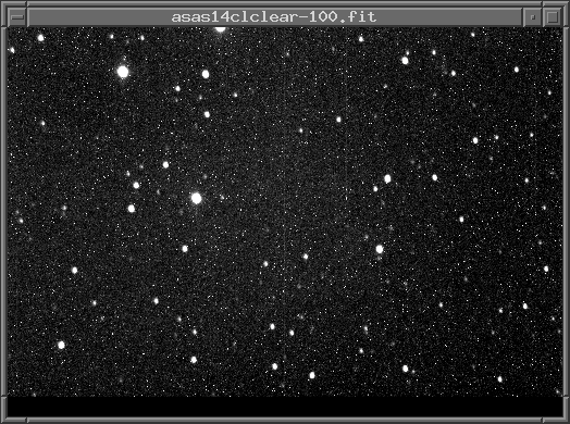
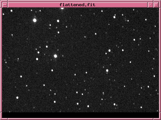
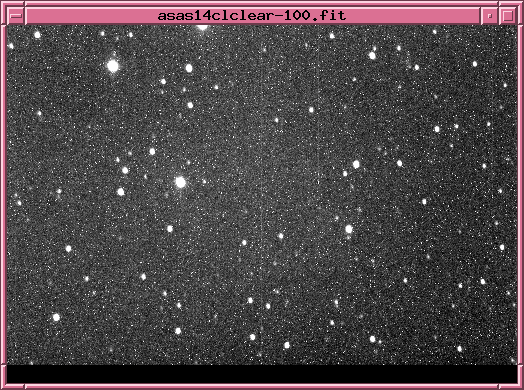
| raw | dark-subtracted | dark-subtracted and flat-fielded |
|

|
|
Connecting to the analysis computer
Each student will log into the same computer to run the image analysis code. The computer's name is spiff.rit.edu, and the instructor will give you the login name and password in class. Your first job is to run the software needed to log into the computer remotely, and set up an X-Windows session so that programs running on the remote computer can display images and text on your laptop's screen.
The exact command(s) will depend on your OS. As a rough guide,
xterm -T spiff -e ssh -Y -l username spiff.rit.edu
where you should replace username
with the actual username, which your instructor will give you
in class. Then type the password which the instructor will provide.
To check that the connection has been made properly, try running this command as soon as you have logged in:
xclock
If, after a short pause, a window pops up on your screen, showing the face of a clock, then all is well, and you may proceed. If not, ask the instructor or a classmate for help. To kill the clock, type "Control-C" (hold down "Control" key and press "c") in the terminal window.
Your next task is to find your special directory (folder) on the analysis computer. Each student will have a directory for that student's own use; all the data you analyze and modify will live inside that directory and its sub-directories. The Unix command ls prints a list of the contents of the current directory. When you have logged into spiff, you should see a prompt that looks something like this:
stu@spiff:~$
If you type ls, you should see that the only two items in this home directory are sub-directories named ast613 and bin. You can move to the directory ast613 by typing the cd command:
cd ast613
If you once again type ls, you will see that THIS directory contains a set of sub-directories:
adler   fall_2022  kelly  malagon   melso   richmond   spr_2025
bloggs  fall_2023  kiely  mcmahon   naylor  rosenberg
cook    finavia    kumar  mcmaster  quinn   solvason
Now, use the cd command once more to change into your own directory. In my case, I would type
cd richmond
In this, your own private directory, you should find a large set of raw FITS files. Those are the items we will analyze.
To begin, let's check some properties of the raw FITS images. There are about 72 images, but each one is pretty small (only 510 x 340 pixels), so the total size of the dataset is only around 38 Megabytes. If you ever happen to delete or mutilate these images, you can grab a fresh set from this zip archive:
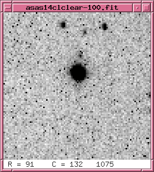
You can print the FITS header of an image in two ways; in the example below, I'll use the image asas14clclear-100.fit.
more asas14clclear-100.fit
buffers asas14clclear-100.fit
Part 1:
When you have answered these questions, please inform the instructor. Look around to see if you can help any of your neighbors.
We will use a suite of image processing programs called the XVista package to examine, modify, and measure properties of the FITS images. XVista is free and open-source, but I don't recommend that you use it unless you want to dive into the source code. But it will allow us to perform some simple analysis for this class.
You can find a short tutorial on some of the XVista commands at
I have set up things for you so that you should not need to carry out the items mentioned in the "A few preliminaries" section. In general, typing the name of a command, followed by "help", will often provide some information on the arguments for the command. For example, try typing tv help .To begin, experiment with the XVista commands and options to make sure you can display an image.
The tv command will create a new window and fill it with the pixel data from a FITS image. In simplest form,
tv asas14clclear-100.fit
You can change the contrast settings with additional arguments; for example, the following command will set pixels less than 1000 to pure black, and pixels greater than (1000 + 300) to pure white.
tv asas14clclear-100.fit z=1000 l=300
I prefer to display images with black stars on a white background, which can be done by using the "invert" argument just once:
tv asas14clclear-100.fit z=1000 l=800 invert
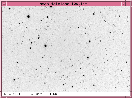
As you move your cursor in this image window, the current pixel location, and the current pixel value, will be shown in the lower-left corner of the window.
You can create a new window which zooms in on the current location of the cursor by pressing the "z" key. For example, if I move my cursor to the bright star near (40, 106), and press "z", I will cause this new window to appear:
If you have a mouse, you can change the contrast settings interactively by pressing and holding the middle mouse button while moving the cursor across the window.
When you are done with a window, you can delete it either by using your OS's window manager -- the little "X" in the upper corner of the image on Windows, or the red dot in the upper corner of the image on Mac OS -- or you can simply right-click while inside the window.
Pick just one of the target images: asas14clclear-100.fit, which I'll call "target image 100" for short. Look at the FITS header of this image and answer the following questions.
Part 2:
When you have answered these questions, please inform the instructor. Look around to see if you can help any of your neighbors.
If we take a picture with the shutter closed, our camera SHOULD record an image which is completely empty -- no signal at all. Right? But CCDs don't work that way. Even if no light hits the silicon, electrons can still be knocked free by thermal motions of the atoms.
Let's find out just how large a signal is created this way.
First, let's display one of the raw, 1-second dark frames:
tv dark1-001.fit z=160 l=100

Note the "salt-and-pepper" appearance of the image, which is due to small variations from one pixel to the next. Some of these variations are due to random noise in the readout process, and in the thermal motions of atoms; but some are systematic, and will appear in every dark frame. One way to measure the pixel-to-pixel variations is with XVista's mn command, which computes the mean and standard deviation of all the pixels in an image:
mn dark1-001.fit
We can reduce the random noise, and enhance the systematic effects, by combining 10 individual 1-second dark exposures to create a "master" dark frame:
median dark1-*fit outfile=master_dark1.fit
We can display this image so it's easy to compare to the individual dark frame (the "xo=600" argument places this new window 600 pixels away from the left edge of your screen).
tv master_dark1.fit z=160 l=100 xo=600

We can compute the statistical properties of this "master" dark image using the mn command on it:
mn master_dark1.fit
Part 3:
There is also a series of 10 dark images with a longer, 30-second exposure time. Use the same steps to create a "master" 30-second dark image, called master_dark30.fit.
If you want to investigate the behavior of the dark current in more detail, the XVista command hist will create a text file with a count of the number of pixels with each pixel value. For example,
    hist master_dark30.fit

		  Mean  adus     207.86
		  Total adus 36043331.000000
		  Max.  adus   25131 at row= 172  col=485
		  Min.  adus  -32454 at row= 157  col=311
		  Total     pixels 173400.000000
		  Overflow  pixels          0
		  Underflow pixels          1
		  Standard deviation =     132.08
		  Median        198  adus  *** warning underflow
		  Mode          198  adus  *** warning underflow


    more master_dark30.his

       0                0 0.000
      29                0 0.000
      30                1 0.000
      31                0 0.000
      62                0 0.000
      63                1 0.000
      64                0 0.000
      97                0 0.000
      98                1 0.000
      99                0 0.000
     141                0 0.000
     142                2 0.000
     143                0 0.000

        (etc.)
When you have answered these questions, please inform the instructor. Look around to see if you can help any of your neighbors.
Creating a master flatfield image
What should happen if we take an image of a blank white, uniformly lit card? We SHOULD see a picture which has the same pixel values everywhere -- nice, uniform, white (or maybe grey) pixels, all the same.
But if you take a real picture with a real CCD, attached to a real telescope, you will usually see something quite different. Something which is NOT uniform at all!
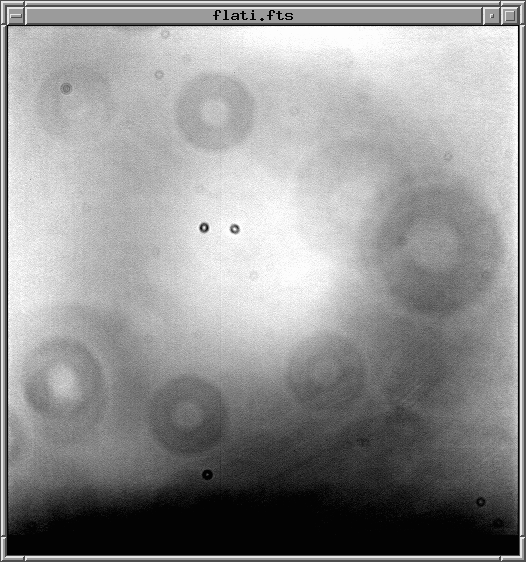
Typically, these "flatfield" images show evidence for several types of defects:
If we can make a map of these defects, then we can correct for them later. Let's try that with data from this evening. I took pictures of the twilight sky, just after sunset, when it was still too bright to show (many) stars. There is a set of 10 images, all with names like flatclear-001.fit.
The procedure for creating the "master" flatfield frame involves two steps:
Let's carry out each step in turn, but pause between them to examine the intermediate products.
Part 4
sub flatclear-001.fit master_dark1.fit outfile=flatclear-001_sub.fit
The result should be a set of new, dark-subtracted images, each with a filename ending in "_sub.fit".
median flatclear-*_sub.fit outfile=master_flatclear.fit
mn master_flatclear.fit
When you have answered these questions, please inform the instructor. Look around to see if you can help any of your neighbors.
Okay, we're ready for the big step: we are going to clean the target images. Our procedure will be equivalent to these mathematical steps:
       Step 1:      subtract appropriate master dark

       Step 2:      divide by a normalized version of master flat
We could also write that, on a pixel-by-pixel basis, we will do this:
                              raw(i,j) - master_dark(i,j)
  clean pixel (i,j)  =   [ --------------------------------- ]  * FLATMEAN
                                   master_flat(i,j)
where FLATMEAN is the mean pixel value in the master flatfield image.
Here are the commands you can run to perform these calculations on the raw ASASSN-14cl images. I'll use just one image as an example, but each student should pick a set of 5 consecutive images (for example, numbers 100 - 120, or 040 - 060) and do this for all 5 of them. The commands I show below will place the "cleaned" images into a sub-directory called "clean"; that will keep things organized for later analysis.
Part 5:
sub asas14clclear-100.fit master_dark30.fit outfile=asas14clclear-100_sub.fit
div asas14clclear-100_sub.fit master_flatclear.fit flat outfile=clean/asas14clclear-100_clean.fit
The result should be that a set of nice-looking images appears in your clean sub-directory. These images should be mostly free of hot pixels, and mostly free of obvious flat-field image defects.
If your images still look crummy, check with the instructor.
When you have answered these questions, please inform the instructor. Look around to see if you can help any of your neighbors.
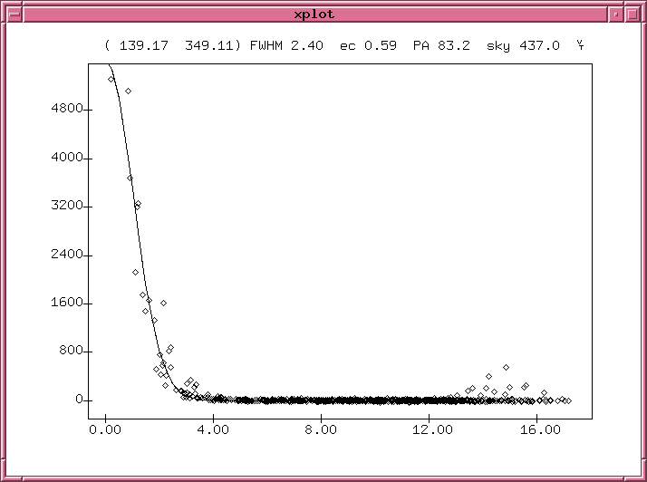
Okay, you have a set of clean images showing ASASSN-14cl and a bunch of other stars. Good! We'll deal with photometry next time, so for now, just measure some image properties and get ready for the science. Choose one of your clean images and examine it to answer the following questions.
Part 6:
Copyright © Michael Richmond.
This work is licensed under a Creative Commons License.