 Copyright © Michael Richmond.
This work is licensed under a Creative Commons License.
Copyright © Michael Richmond.
This work is licensed under a Creative Commons License.
First, a word on the format of this tutorial text. Scattered throughout the document will be examples of commands you could type, and the results of those commands. I will put blocks of such interaction with the computer in sections of text which are indented and shown in a different font. For example, to show how one can list all the files in the current directory,
     % ls

     dark1-001.fit    dark120-008.fit   flatr-004R.fit   m109_r-011R.fit
     dark1-002.fit    dark120-009.fit   flatr-005R.fit   m109_r-012R.fit
     dark1-003.fit    dark120-010.fit   flatr-006R.fit   m109_r-013R.fit
     dark1-004.fit    dark120-011.fit   flatr-007R.fit   m109_r-014R.fit
     dark1-005.fit    dark30-001.fit    flatr-008R.fit   m109_r-015R.fit
     dark1-006.fit    dark30-002.fit    flatr-009R.fit   m109_r-016R.fit
     dark1-007.fit    dark30-003.fit    flatr-010R.fit   m109_r-017R.fit
     dark1-008.fit    dark30-004.fit    m109_r-001R.fit  m109_r-018R.fit
     dark1-009.fit    dark30-005.fit    m109_r-002R.fit  m109_r-019R.fit
     dark1-010.fit    dark30-006.fit    m109_r-003R.fit  m109_r-020R.fit
     dark120-001.fit  dark30-007.fit    m109_r-004R.fit  m109_r-021R.fit
     dark120-002.fit  dark30-008.fit    m109_r-005R.fit  m109_r-022R.fit
     dark120-003.fit  dark30-009.fit    m109_r-006R.fit  m109_r-023R.fit
     dark120-004.fit  dark30-010.fit    m109_r-007R.fit  m109_r-024R.fit
     dark120-005.fit  flatr-001R.fit    m109_r-008R.fit  m109_r-025R.fit
     dark120-006.fit  flatr-002R.fit    m109_r-009R.fit
     dark120-007.fit  flatr-003R.fit    m109_r-010R.fit
The % character is the computer's command-line prompt. I typed the command ls, then pressed the "Enter" key. The computer replied with a list of all the files in the directory. I have added a blank line between my command and the computer's response for clarity.
In order to use any of the XVista programs, I need to set the environment variable SYM_TABLE to the name of a file which I can read and write. I usually pick a file in my home directory with a name which is unlikely to be used for other purposes. So, when using the bash shell, I type
% export SYM_TABLE=$HOME/.sym
If I am using a csh-like shell, the syntax for setting an environment variable is slightly different:
% setenv SYM_TABLE $HOME/.sym
A number of the XVista programs will read and write short text lines to this file. It is all plain ASCII, so you can edit it with any ordinary text editor if you wish.
You can type one of these commands manually at the very start of a session of using XVista, if you wish. It is probably more convenient to place these commands into a file which is automatically executed when you log into the computer, or whenever you spawn a new shell process. Since I use the "bash" shell, I have added to my .bash_profile file one line to set this environment variable every time I log in.
There is one last step that is necessary if you plan to use the tv command to display FITS images. You must run this command first, just once, at the start of a session of XVista commands:
% propinit
The propinit command initializes some information in the X Windows server which is used to pass information between several XVista processes. That is, if you first run tv to create a window showing some image, and then use the box command to define a box interactively by moving the cursor around in the displayed image, the box process needs to ask the tv process exactly what (row, col) pixel coordinates correspond to the cursor's location. If you forget to run propinit at the start of your session, the tv command will not open a window, but fail with a cryptic error message. It is not so easy to automate this step, since the propinit command can succeed only when run under X Windows; many users will log into a computer in text mode, and only later start X Windows.
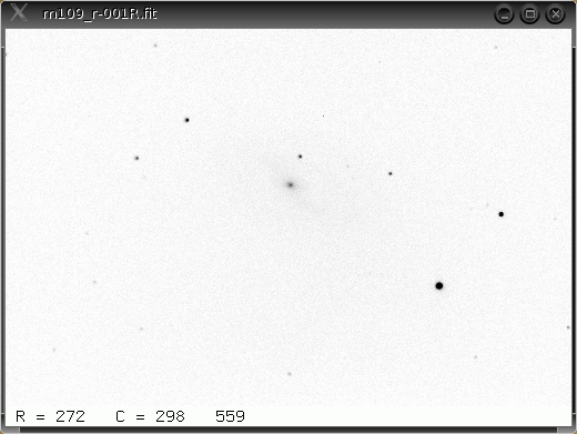
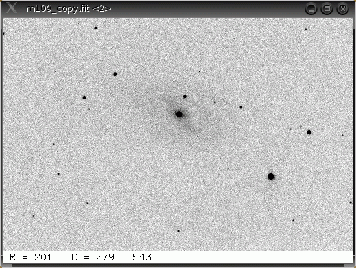
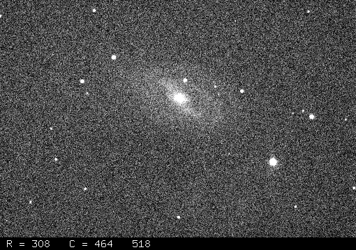
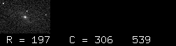
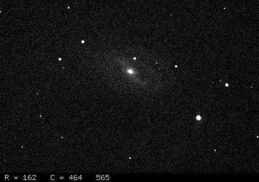
One very common task is turning a raw CCD image into a "clean" picture, by subtracting the dark current and dividing by an appropriate flatfield. In this example, we'll start with an image of M109 taken with the RIT Observatory's 12-inch telescope and SBIG ST-8E CCD camera. Below is a picture of the raw, 30-second, R-band image.

Our plan is to
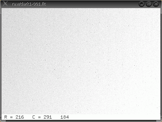
Step 1: create a median 1-second dark frame from a set of 10 individual 1-second-long dark frames. Below is a single 1-second dark image:
To combine 10 such raw frames into a master 1-second-long dark frame, we use the XVista command median. (The % character is the shell prompt -- I actually typed the characters starting at "median")
% median dark1-*.fit outfile=dark1_master.fit nomean
The first argument to this command is a list of input files; we use a Unix wildcard character, the asterisk *, to match all the files with names like "dark1-001R.fit", "dark1-002R.fit", etc. The outfile= argument tells the program the name of the file into which to write the newly created median image. The nomean keyword at the end of this command instructs the program not to scale each image to have a common mean value, but to find the median value at each pixel location in each input file, just as they are.
The master dark looks very much like any of the individual dark frames. It has slightly lower noise, and any cosmic rays or other events which appear in a single frame will be removed in the median output file.
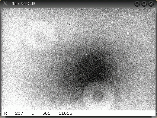
Step 2: subtract the 1-second master dark frame from each of the raw flatfield images. A single raw flatfield image is shown below.
Since the typical pixel values in the flatfield frame are much larger than those in the dark frame, we won't be able to see much of a difference after we subtract the dark frame. I'll use the mn command to compute the statistics of the flatfield frame before and after the subtraction to verify that we really did change the flatfield frame.
      % mn flatr-001R.fit

      mean=11533.43 rms=119.72 sum=1999896972 npixels=173400

      % sub flatr-001R.fit dark1_master.fit

      % mn flatr-001R.fit

      mean=11354.57 rms=123.53 sum=1968882618 npixels=173400
Good. The mean value of this flatfield image has decreased by about 180 counts. That is exactly the mean value of the master dark image.
There are ten raw flatfield images in the directory. I could type ten commands to subtract the master dark frame from each one in turn, or I could write a simple script so that the computer did the drudgery. I could do it in bash like so:
     % for i in flatr-0*.fit
       do
         sub $i dark1_master.fit
       done
I could also write a very short and simple script in some other language, such as Perl or TCL, to do the same thing. At the end of this tutorial is a link to a Perl script I use to subtract dark frames from similar data.
Step 3: combine the dark-subtracted flatfield frames to create a master flatfield image. Once again, the median program does the job. This time, however, we include different options.
     % median flatr-*.fit outfile=flatr_master.fit iqm verbose
     file  flatr-001R.fit has mean  11354.57   (in symbol table)
     file  flatr-002R.fit has mean  23922.00   (in symbol table)
     file  flatr-003R.fit has mean  23050.00   (in symbol table)
     file  flatr-004R.fit has mean  22143.00   (in symbol table)
     file  flatr-005R.fit has mean  21155.00   (in symbol table)
     file  flatr-006R.fit has mean  20395.00   (in symbol table)
     file  flatr-007R.fit has mean  19640.00   (in symbol table)
     file  flatr-008R.fit has mean  18827.00   (in symbol table)
     file  flatr-009R.fit has mean  18095.00   (in symbol table)
     file  flatr-010R.fit has mean  17401.00   (in symbol table)
        median file flatr_master.fit: up to row   320 out of   340
The iqm argument tells the median program not to compute a true median at each pixel location, but instead to calculate the interquartile mean. I find that in some case, this statistic yields better results than a median. The verbose option causes the program to print out some of its results as it goes. The default action of median is to scale all the input images to a common level before combining them (since we did not specify the nomean option). We therefore are shown the mean values of each of the input images as it computes them. We are also shown a single line at the bottom which counts the rows of the median image as it is created. Back in the old days, when computers were slow, this would provide a useful check on how much time it would take to finish the job.
Below is the output, master flatfield image.
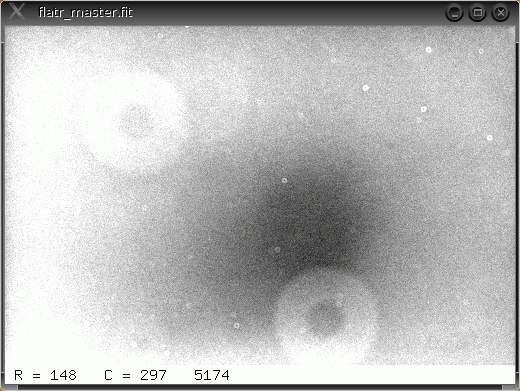
As you can see, it looks very much like a single raw image, but is somewhat smoother and less noisy.
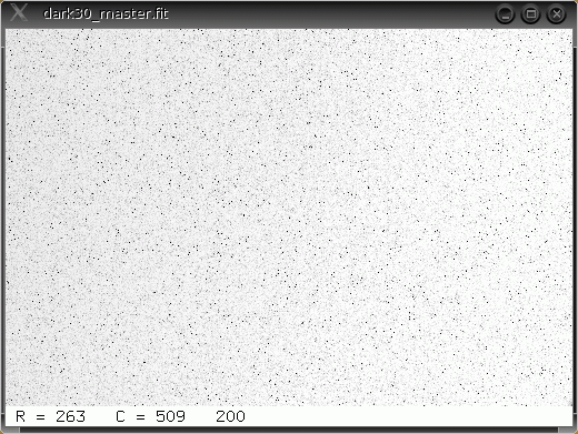
Step 4: create a median 30-second dark frame. We will use this to remove the thermal signal from our 30-second long target images. typed the characters starting at "median")
% median dark30-*.fit outfile=dark30_master.fit nomean
The result shows a good many hot pixels.
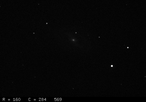
Step 5: subtract the median 30-second dark frame from our target images. We again use the sub command.
% sub m109_r-001R.fit dark30_master.fit
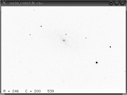
If all goes well, this should have removed all the hot pixels from our target image. Let's see -- compare the dark-subtracted image below with the original raw image at the top of this section. Here's the dark-subtracted version, displayed with the command
% tv m109_r-001R.fit z=517 l=1000
The z=517 argument specifies that image pixels with values 517 (or lower) should be displayed as pure white, and the l=1000 -- that's the letter "ell" before the equals sign -- states that pixels with values 1000 greater (i.e. 517+1000=1517) and higher should be displayed as pure black. In between these two limits, pixels are shown as shades of grey.
Good! That does look better.
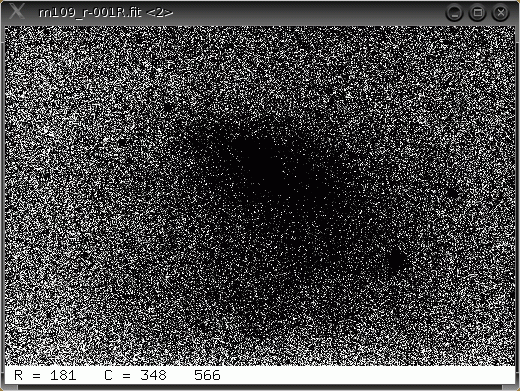
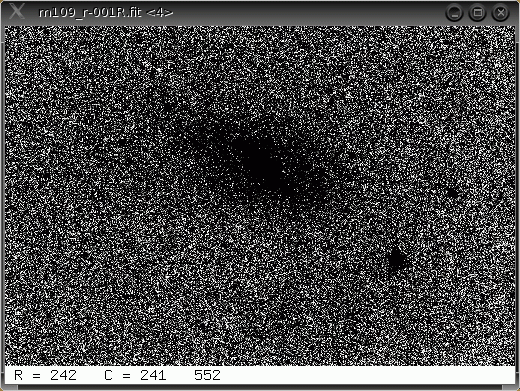
However, if we display this image with a very hard contrast setting, like so:
% tv m109_r-001R.fit z=517 l=20
then we emphasize features in the pixels with values between 517 and 517+20 = 537; in other words, pixels which contain no light from stars or galaxies, but just background sky. Now we see that the background is not uniformly bright: the illumination drops off in the corners of the field.
Step 6: divide the target frame by the master flatfield image. This should correct the slight variations in illumination across the image. To do this right takes two steps. First, we need to calculate the mean value of the flatfield image we will use to correct the target frames.
     % mn flatr_master.fit

     mean=5102.02 rms=48.54 sum=884689773 npixels=173400
This mean value is stored in the symbol table for future reference. We can look at all the entries in the symbol table with the xlet command. If we provide no arguments, it shows us the entire table.
     % xlet

     mn_flatr-001R.fit= 11354.57
     mn_flatr-002R.fit= 23922.00
     mn_flatr-003R.fit= 23050.00
     mn_flatr-004R.fit= 22143.00
     mn_flatr-005R.fit= 21155.00
     mn_flatr-006R.fit= 20395.00
     mn_flatr-007R.fit= 19640.00
     mn_flatr-008R.fit= 18827.00
     mn_flatr-009R.fit= 18095.00
     mn_flatr-010R.fit= 17401.00
     mn_flatr-011R.fit= 14749.00
     mn_flatr-012R.fit= 14111.00
     mn_flatr-013R.fit= 13505.00
     mn_flatr-014R.fit= 12962.00
     mn_flatr-015R.fit= 12417.00
     mn_flatr.fts= 24965.79
     mn_dark1_master.fit=   178.86
     mn_flatr_master.fit=  5102.02
The final entry is the mean value of this master R-band flatfield frame.
Once we have computed this mean value, we can use the div command to divide the target image by the master flatfield image; adding the flat keyword causes the div program to multiply the result by the mean value of the flatfield frame before finishing.
     % div m109_r-001R.fit flatr_master.fit flat

     Mean is 5102
The div command prints out the value by which
it scales the result as a reminder that it is doing
a flatfield division.
Thus, we should get a final image which has the same average value as the input image, but with variations in the background level smoothed out. Let's look at the final image, using a soft contrast setting, then a hard one.
% tv m109_r-001R.fit z=517 l=1000
% tv m109_r-001R.fit z=517 l=20
I've placed a sample Perl script which does this flatfielding step to a number of target images at the end of this tutorial.
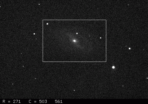
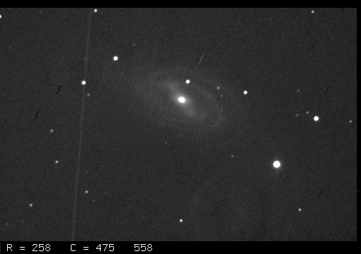
Sometimes, all we care about is a section of an image. In this picture of M109, the galaxy occupies just a portion of the entire frame. Let's create a version of the image which consists only of this portion.
First, I'll make a copy of the clean image and display it.
     % cp m109_r-001R.fit m109_copy.fit

     % tv m109_copy.fit z=500 l=200
I will use the box command to define a rectangular box which includes only portions of the image around the galaxy. One way to define the box is interactively: type
     % box 1 int

     click and hold Left for center of box, then drag and release
     box #1 cr=142 cc=257 nr=154 nc=176
and follow the printed instructions: move the cursor to the center of the desired area, then click-and-hold the Left mouse button. While holding the button down, drag the cursor and watch as a box expands to follow the cursor. When the box reaches the desired size, release the Left button. When you finish, the program will print the number (here number 1) and the coordinates of the box you have defined.
Another way to define a box is to provide its coordinates explicitly. You can define the center and size:
     % box 2 cr=150 cc=240 nr=100 nc=100

     box #2 cr=150 cc=240 nr=100 nc=100
or you can provide the starting row and col, plus size:
     % box 2 sr=80 sc=120 nr=100 nc=100

     box #2 cr=130 cc=170 nr=100 nc=100
In either case, the program will echo the final coordinates of the box (using center plus size format) to the screen when you are done.
You can see a list of all known boxes by typing the box command with no arguments:
     % box

     box #1 cr=142 cc=257 nr=154 nc=176
     box #2 cr=130 cc=170 nr=100 nc=100
You can redefine a box's coordinates at any time; there is no need to delete a box.
Once a box has been defined, you can use the box program with the show argument to display the box on any images which are active. Just type
% box 1 show
to see box number 1 inscribed on the image, like this:
If you repeat the command,
% box 1 show
then the box will be drawn in reverse colors -- which will cancel the original box and cause it to disappear. If you execute the command a third time, the box shows up again; a fourth time, it disappears again. The mode of drawing will toggle between normal and inverted every consecutive time you "show" a box on one particular image.
What can I do with a box? For one thing, many of the XVista commands can be told to act only on the portion of an image which lies within a particular box. For example, to compute the mean value of pixels inside box number 1 only, I can type
     % mn m109_copy.fit box=1

     mean=548.88 rms=25.66 sum=14876783 npixels=27104
The window command is designed to crop an image. It throws away all pixels which lie outside the given box. So, if I execute this command and then display the image again,
     % window m109_copy.fit box=1

     % tv m109_copy.fit z=500 l=200

We can display a small image with a large "zoom factor" by using the tv command with the zoom= option:
% tv m109_copy.fit z=500 l=200 zoom=4
The tv command displays a FITS image. You'll probably use it a lot. Let's look at the many options and features to this command.
If you type the name of this command (or almost any XVista command) following by the single argument help, you'll be shown a list of the command-line options.
     % tv help

     usage: tv file [span] [zero] [box=] [l=] [z=] [xo=] [yo=]
        [zoom=] [hist] [dither] [nofork] [invert] [live=] [falsecolor] [help]
Arguments listed inside square brackets, such as [box=], are optional. Arguments listed without square brackets, such as file, are required, and must appear in the order given. So, for the tv command, the first argument must be the name of the FITS image you wish to display.
Let's provide the minimum required information: just the image name. Two things happen: a single line with some information is printed to the screen, and a new window appears with a picture of the image.
     % tv m109_r-001R.fit

     Autospan= 256 zero= 519
The two numbers printed in response to our command are the "zero" and "span" values chosen to define the translation of FITS image pixel values to display pixel values:
If the user does not supply values for these two parameters on the command-line, the tv command will try to guess reasonable values by examining a small number of random pixels within the image. Those random pixels will change each time you run the tv command, so the displayed image will look a bit different if you type the command over and over again without specifying the arguments.
You can emphasize faint features by using a smaller span value. These two versions of the command are equivalent: both specify that
     % tv m109_r-001R.fit z=510 l=100

     % tv m109_r-001R.fit 100 510
On the other hand, if we want to hide faint features and emphasize only the bright objects in an image, we can use a large value for the "span", like so:
% tv m109_r-001R.fit z=510 l=1500
Some people like to examine pictures in "reverse video" or "photographic negative" form, in which regions of little light are shown as white and regions of high light intensity are shown as black. You can use the keyword invert to toggle back and forth between "normal" and "reverse" video modes. The first time we type it, we will get a "reverse" mode picture.
% tv m109_r-001R.fit z=510 l=300 invert

Note that you may have to move your cursor into the displayed window for the colors to appear reversed. Depending on your hardware setup, this may cause the colors in all OTHER open windows on your monitor to reverse, too.
From this point on, if you display more images using the tv command without specifying the invert, they will all be shown in "reverse video" mode. The XVista package remembers (in its SYM_TABLE file) the fact that you requested "reverse video" mode, and continues to use it. In order to show images in "normal" mode again, with white stars on a black background, you should supply the invert keyword again -- just once. Don't use invert each time you run tv unless you want to alternate between "normal" and "reverse video" modes continuously!
By default, every time you run tv, it will draw a new image window in the upper-left corner of your screen. You can use the xo= and yo= arguments to move the location of the window to a different location. For example, my screen is currentl 1280x1024 pixels in size. If I type
% tv m109_r-001R.fit xo=500 yo=200
then the window will be drawn starting 500 pixels away from the left
edge of the screen and 100 pixels below the top, as shown below
(click on the picture below for a full-sized screenshot).

Images will remain displayed on your screen until you explicitly tell them to disappear. You can do this in several ways:
There may be times when you do NOT want the tv process to fork and run in the background; for example, if you are running a script of some sort. In that case, add the keyword nofork to the command line, and you won't be returned to the shell until you've killed the display window. Or, if you supply the live= option with some number, say, live=10, the displayed window will remain for the given number of seconds (10, in this case), then commit suicide and return command to the shell.
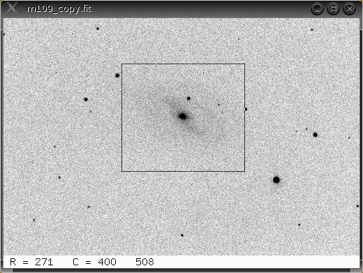
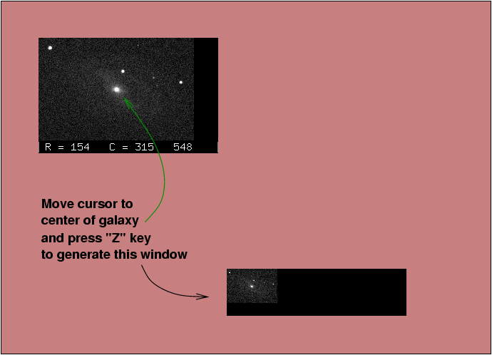
The zoom= option allows you to display an image scaled up in size by an integer factor, or scaled down in size by a reciprocal integer. Consider our picture of M109. I'll draw a box around the galaxy (see the section describing boxes ) and call it box number 1.
     % tv m109_r-001R.fit z=510 l=300

     % box 1 int

     box #1 cr=140 cc=256 nr=144 nc=218
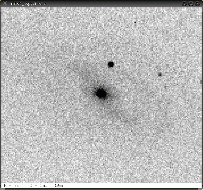
Now, I can display just this section of the image in an expanded fashion: specifying box=1 and zoom=3 will create a window in which each image pixel is drawn as a 3x3 clump of dots on the monitor.
% tv m109_r-001R.fit z=510 l=300 box=1 zoom=3
On the other hand, I can display a very small version of the image by giving a zoom factor less than 1; fractions are rounded to the nearest reciprocal integer.
% tv m109_r-001R.fit z=510 l=300 box=1 zoom=0.33
Note that the window created to hold the displayed image is, in this case, much wider than the image itself. The window will always be drawn wide enough to hold the cursor information, shown below the picture. That data is
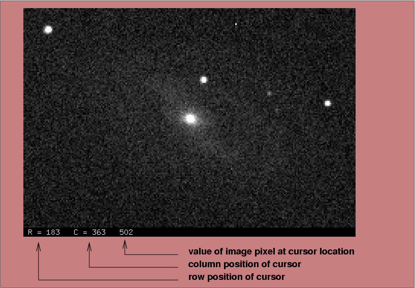
The cursor information will be updated continuously as you move the cursor around in an image window. There may be times when you want to note the position of a star, so that you can type it into some other window or application. If you simply move the cursor away from the image window to your other application, the (row, col) position will change -- very annoying. If you Left-Click once while in the image window, the cursor information will "freeze", so that you can move over to another window without losing it. The image will remain in "frozen" state until your Left-Click again. Every Left-Click toggles the window between "frozen" and "active" states. If you have several tv windows open, they will all "freeze" or "thaw" together.
Please note that the interactive keyboard commands described below will only work in an "active" window; none will occur in a "frozen" window. Some window managers force you to click on a window to bring it to the foreground as well. You'll have to figure out for yourself just how many Left-Clicks it may take to change the state of a window.
Keyboard actions inside the tv window
If you move the cursor to a displayed image window which is in the "active" state, then the following keys cause some action:
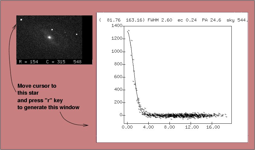
The new window shows the central (row, col) of the fitted gaussian, its FWHM, eccentricity and position angle (in degrees), and the local background "sky" value used in the calculation. The fitting procedure is controlled by the XVista symbols profile_boxrad and profile_fitrad.
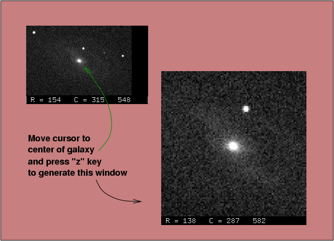
The new window may sit on top of the original image; if so, just move it out of the way.
The new window may sit on top of the original image; if so, just move it out of the way.
mean=635.78 rms=221.77 sum=76929 npixels=121
On the other hand, if I point to a blank region
near the upper-right hand corner of the image, I see printed
to my terminal
mean=540.91 rms=15.88 sum=65450 npixels=121
If I now type the command box, which lists all the known boxes, I should see box number 9 appear, with a location in the upper right-hand corner of the image.
             % box

             box #9 cr=78 cc=353 nr=11 nc=11
82.17 163.19 0.246 0.744 1.000
The numbers here are
                % xlet curveofg_npoints=5
                % xlet curveofg_r1=2
                % xlet curveofg_r2=4
                % xlet curveofg_r3=6
                % xlet curveofg_r4=10
                % xlet curveofg_r5=20
If I again move to the same star and press the c key, I see printed to my terminal
81.75 163.17 0.757 1.003 1.022 0.999 1.000
which tells me that all the light from this star is concentrated within a radius of 4 pixels.
( 81.74 163.16) flux 10759.4 npix 78.9 mag 14.921 sky 545.0 [ 5.0 10 20]
The numbers here are
The XVista symbol aperture_radius sets the size of the circular aperture. The symbols aperture_innersky and aperture_outersky set the boundaries of the annulus used to compute the local background value. The aperture_magzero symbol is used in the equation to convert counts to an instrumental magnitude, like so:
mag = aperture_magzero - 2.5*log10(counts)
The a key is very handy for making quick and dirty estimates of the relative magnitudes of stars in an image. If I use it when pointing to the star at upper-left in the sample image, for example, and then again when pointing to the star at central right edge, I see printed to my terminal
               (  81.74  163.18) flux  10760.7 npix  78.9 mag 14.920  sky  545.0  [ 5.0 10 20]
               ( 129.97  346.37) flux   5190.8 npix  78.3 mag 15.712  sky  543.0  [ 5.0 10 20]
which tells me that the star in the upper-left corner is about 0.8 mag brighter.
Mouse actions inside the tv window
The three mouse buttons perform distinct actions while the cursor is inside an image-display window.
For example, given an original image given by
% tv m109_r-001R.fit z=510 l=600 box=1
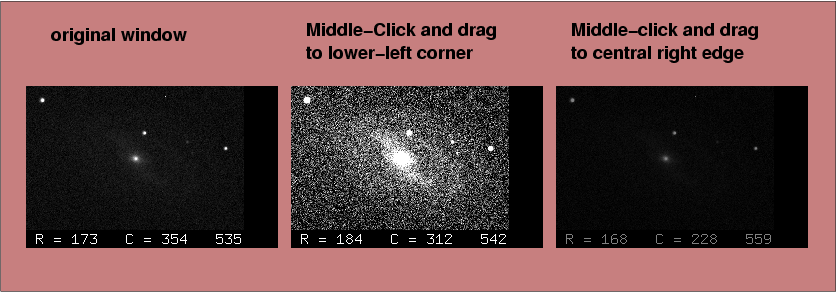
The changes will be reflected in all open tv windows simultaneously. They may also cause the colormap to shift for the entire screen, including windows belonging to other applications.
Some X Windows configurations do not allow user programs to modify the colormap. On those systems, the Middle Button does nothing.
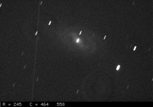
Sometimes, you may take many images of the same object. In theory, combining the images should yield a picture which shows fainter details than any of the individual frames. In practice, it may take a bit of work to achieve the desired results.
The trouble is that the individual frames may not be perfectly aligned with each other. For example, I have a set of 15 images of the galaxy M109 taken one right after the other. Because the telescope didn't track the motion of objects through the sky perfectly, objects slowly creep across the field throughout the sequence. Below are portions of a few of the frames in the series.

I can try to add them all together, using the add program, but it won't be pretty. Note the arguments to add: first must come all the input file names, then the optional arguments. I specify the name of the output, co-added file, and I also request that the sum be normalized by the number of input files.
     % add m109_r-00?R.fit m109_r-01[01234]R.fit outfile=sum.fit norm

     % tv sum.fit z=530 l=200
Yuck. That didn't work.
What I need to do is shift the images so that the stars in each one align with one particular image, which I'll call the template. When all the images have been shifted, then we can add them together. I'll choose image number 1, with name m109_r-001R.fit, to be the template. To figure out the shifts, I'll use the bright star marked "A" in the picture below.
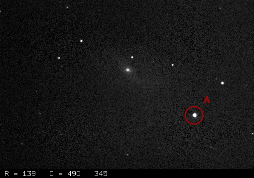
By displaying each image in turn, moving the cursor to the location of this star, and pressing the a key, I can build up a list of the position of star A in each image. Below are a few entries from such a table.
       image        row  col         row-row1    col-col1
   ---------------------------------------------------------
        001       230.88  390.44       0.00        0.00
        002       230.18  390.91      -0.70        0.47
     ...
        005       227.83  393.03      -3.05        2.59
     ...
   ---------------------------------------------------------
Let's pick image number 5, with full name m109_r-005R.fit, as an example. Star A has moved by -3.05 pixels in the row direction (vertically) and by 2.59 pixels in the col direction (horizontally), relative to its position in image number 1. In order to shift the features in image 5 so that they match image 1, I use the imshift program like so; note that I create a copy of the original image number 5, since the imshift program overwrites its input file by default.
     % cp m109_r-005R.fit shifted_005.fit

     % imshift shifted_005.fit dr=3.05 dc=-2.59
Below is an animated GIF which should show a little movie, alternating between the fiducial image number 1 and the shifted version of image number 5. You may need to click on the image to activate the motion. As you can see, the shifted version does match up quite nicely with the fiducial.
So, if we do this for each of the 15 images, one by one, we will have a set of aligned images with names like shifted_001.fit, shifted_002.fit, ... shifted_015.fit. We can then add them together in two ways: a simple summation (with normalization) via add:
% add shifted_*.fit norm outfile=shift_sum.fit
The result does indeed show fainter stars than any of the individual images:
% tv shift_sum.fit z=530 l=200
However, note several artifacts: there was a satellite trail through one of the fifteen images, and it shows up in this sum. There are also several short streaks due to hot pixels which weren't exactly removed by our dark subtraction.
If we combine the shifted images with the median command, we can get rid of some of these artifacts: they will appear at a particular (row, col) location in just a single image, so the median value at each (row, col) will avoid them.
     % median shifted_*.fit outfile=shift_median.fit

     % tv shift_median.fit z=530 l=200

The only remaining artifact is the dust ring at the bottom right. The filter, or the dust speck causing the ring, must have shifted slightly between the time we took the flatfield images and the time we acquired the target images.
It is possible to use the tv command to measure the positions and instrumental magnitudes of stars in an image: just display the image, move the cursor to a star, and press the a or c or r key. This could become tedious if one wants to measure the properties of tens or hundreds of stars in a single image ... or stars in tens or hundreds of images.
The XVista package includes several programs which are designed to perform simple measurements of stars automatically. They work only in limited situations:
The programs are modelled on the description of some of the routines included in the original version of DAOPHOT, written by Peter B. Stetson and published in
DAOPHOT - A computer program for crowded-field stellar photometry , PASP vol 99, 191 (1987).
but, again, the routines included in XVista do NOT include PSF-fitting. They are instead simple analogs to the FIND and PHOT routines, which are only the starting points to more sophisticated functions in DAOPHOT.
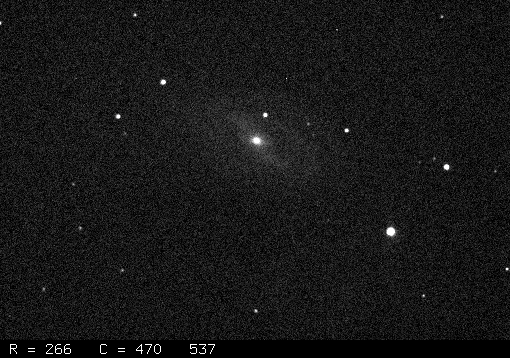
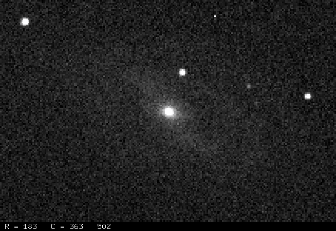
Let me introduce them with a short example. Given the cleaned image of M109 we have used in other examples,

we can find, then measure, the bright stars with the following sequence of commands.
     % sky m109_r-005R.fit

     sky=539 skysig=16.90

     % stars m109_r-005R.fit minfwhm=1.5 maxfwhm=3.5 minsig=10 outfile=m109.coo

     % phot m109_r-005R.fit infile=m109.coo outfile=m109.pht aper=3

     % cat m109.pht
         1   11.27  136.94    543   6.58   16.718  0.068    0
         2   13.09  443.81    541   6.86   17.503  0.131    0
         3   19.81    1.33    542   6.85   15.875  0.034    4
         4   78.74  165.58    551   6.82   15.045  0.018    0
         5  111.47  267.56    563   7.23   15.583  0.027    0
         6  112.98  120.27    547   7.14   15.664  0.029    0
         7  126.86  348.89    548   6.65   15.764  0.031    0
         8  163.38  448.75    544   6.54   13.770  0.008    0
         9  227.86  393.00    548   6.61   11.547  0.002    0
        10  292.04  425.57    543   6.16   17.448  0.125    0
        11  307.64  257.79    544   6.53   16.942  0.082    0
Now, let's go over each of the steps.
     % hist m109_r-001R.fit

     Mean  adus     542.25
     Total adus 94025379.000000
     Max.  adus   32474 at row= 231  col=390
     Min.  adus    -107 at row= 120  col= 86
     Total     pixels 173400.000000
     Overflow  pixels          0
     Underflow pixels          1
     Standard deviation =     168.42
     Median        539  adus  *** warning underflow
     Mode          536  adus  *** warning underflow
This will create a text file with the same name as the image, but with the final extension replaced with ".his"; in this case, m109_r-001R.his. This text file has two columns of data: pixel value in column 1, number of pixels with that value in column 2. I show below a plot of this histogram, which I made using gnuplot .
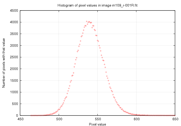
The sky program returned a value of 539 counts, with a standard deviation of 17 counts. That does indeed look like a good representation of the distribution of pixel values. Not only does the sky program print these results to the terminal, but it also sets several variables in the symbol table for future reference: in this example, the sky symbol is set to 539, and the skysig symbol is set to 16.90.
% stars m109_r-005R.fit minfwhm=1.5 maxfwhm=3.5 minsig=10 outfile=m109.coo
where the first argument must be the FITS image we are
examining. The minfwhm= and maxfwhm= arguments
provide lower and upper limits (in pixels) to the FWHM
(full-width at half-maximum)
of objects which will be called stars and included in the output.
The next argument, minsig=, states how bright
a peak pixel must be to trigger the decision process:
in this case, 10 times the skysig value above
the sky value.
If arguments for sky and skysig are not
provided on the command-line, the program will look into
the symbol table to find them. In our case, these
symbols have values sky=539 and skysig=16.90,
so any pixel with (539 + 10*16.90) = 708 counts, or more,
will be considered as a possible star.
The final argument above tells the stars program to write its results to a file called "m109.coo"; by default, results are printed to the terminal. The output is an ASCII list of objects which have passed all tests and qualify as stars, in the following format:
         1   11.27    136.94     203    2.926    -0.030    0.650
         2   13.09    443.81     189    2.285    -0.125    0.836
         3   19.81      1.33     529    2.821    -0.063    0.563
         4   78.74    165.58    1332    2.723     0.052    0.743
         5  111.47    267.56     770    2.779    -0.051    0.742
The columns are
                                       xwidth - ywidth
                    roundness =  2 * (-----------------)
                                       xwidth + ywidth
Adding the keyword show to the stars command will cause crosses to be drawn on any open image window at the location of each object as it is found. So, the following sequence of commands:
     % tv m109_r-001R.fit

     % stars m109_r-001R.fit minfwhm=1.5 maxfwhm=3.5 minsig=10 outfile=m109.coo show
cause the tv window to look like this:

You can annotate an image in a slightly different way after the fact. The marks program will draw numbers at specified locations on an image. I very often use it to display the output of the stars command in the following way:
% marks m109.coo num=1 row=2 col=3
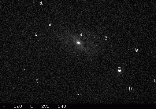
We can now see at a glance that the bright star in the lower-right portion of the image is number 7 in the list produced by stars (or by phot in the section below).
% phot m109_r-005R.fit infile=m109.coo outfile=m109.pht aper=3
The first argument is the name of the image on which stars will be measured. The remaining arguments can appear in any order. The source of the positions is given by infile=; the format of this file must be exactly that produced by the stars program. The output will be printed to the terminal by default, but can be directed into a text file via the outfile= argument. The final argument shown above, aper=3, sets the size of the circular apertures used to measure starlight: 3 pixels in radius.
The algorithm is simple: a circle of the given size is drawn around the central position of a star. The light from all pixels which lie within that circle -- including a fraction of the pixels which are transected by the circle's edge -- is added together. The program then computes the contribution of the background to this sum: by default, it uses an annulus surrounding the star, with radii set by the skyinner= and skyouter= arguments, to determine a local background value; but one can also specify a single fixed background value for all objects with the sky= option. After subracting the background from the integrated light, the program converts the flux to an instrumental magnitude via the usual equation
mag = mconst - 2.5*log10(flux)
The program also attempts to estimate the uncertainty
in this measurement; by default, it uses photon
statistics, which will be accurate only if the user
supplies good values for the gain= and readnoise=
arguments. However, if the user gives the
empscatter keyword, the uncertainty will be
estimated using empirical heuristics.
In most cases, the program will underestimate the
actual uncertainty in measured instrumental magnitudes.
The output of the phot program is another ASCII table with line per object:
         1   11.27  136.94    543   6.58   16.718  0.068    0
         2   13.09  443.81    541   6.86   17.503  0.131    0
         3   19.81    1.33    542   6.85   15.875  0.034    4
         4   78.74  165.58    551   6.82   15.045  0.018    0
         5  111.47  267.56    563   7.23   15.583  0.027    0
The columns are
If the user supplies several aper= values on the command line, like this:
% phot m109_r-005R.fit infile=m109.coo outfile=m109.pht aper=3 aper=4 aper=6
then the program will make measurements through each of the given apertures, producing a longer list of output, with pairs of (mag, uncert) values for each aperture in turn:
       1   11.27  136.94    543   6.58   16.718  0.068  16.646  0.082  16.568  0.110    0
       2   13.09  443.81    541   6.86   17.503  0.131  17.454  0.162  17.401  0.223    0
       3   19.81    1.33    542   6.85   15.875  0.034  15.790  0.040  15.756  0.055    4
       4   78.74  165.58    551   6.82   15.045  0.018  14.956  0.020  14.929  0.027    0
       5  111.47  267.56    563   7.23   15.583  0.027  15.521  0.032  15.505  0.045    0
The "quality flag" serves to mark any cases in which the measurement process suffered some problem: for example, if a star was close to the edge of an image, or near a region of the image marked as having a defect. See the phot man page for details.
At the end of this tutorial is a Perl script, stars.pl , which I use frequently: it loops over a series of images, running in turn the sky, stars, and phot programs on each one to generate text files with stellar positions and instrumental magnitudes.
Once you have such a series of text files, one per image, you might use the ensemble package to analyze them all.
Copyright © Michael Richmond.
This work is licensed under a Creative Commons License.