This report describes the results of my analysis of some of the Oct 2013 commissioning data. It is not the complete report, but a short note on results so far.
This report focuses on a set of images of the field of MASTER OT J061335.30+395714.7, a cataclysmic variable star. I analyze the measurements of stars in this uncroweded field in a set of 10 consecutive 60-second exposures.
All the data were taken in 4-amp readout mode.
Contents:
I examined the overscan columns of a number of images in this dataset. In Feb 2013, I found that there was a trend for the overscan pixel values to decrease slightly from one end of the image to the other. In these images, I found no such trend: the overscan pixel values were stable within each image, for all 4 amplifiers.
However, I did see that in most images, the very first row of data -- both overscan and target pixels -- and/or the very last row -- both overscan and target pixels -- were different. These first and/or last rows had pixel values that were higher or lower than all the other rows.
The overscan regions for each amplifier had slightly different pixel values.
   amplifier      overscan value
  --------------------------------
      1               3084
      2               2918
      3               2932
      4               3112
  --------------------------------
I subtracted the mean overscan value from each image quadrant before all subsequent analysis.
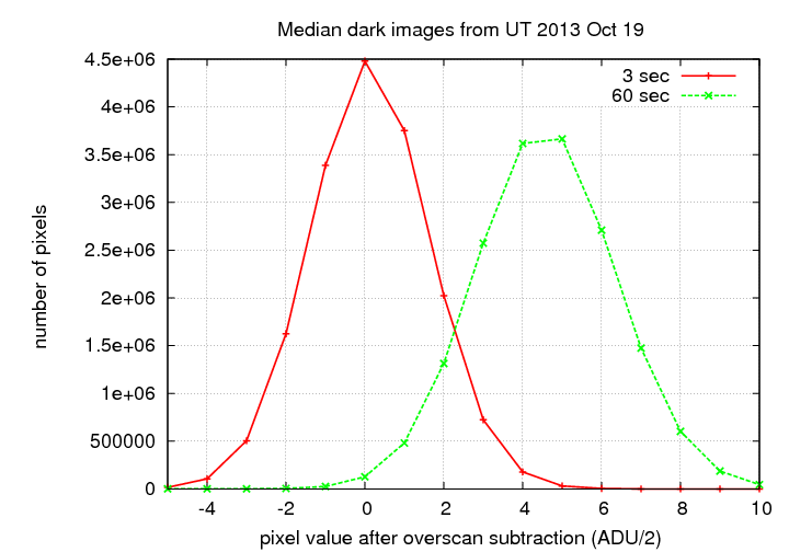
I created master dark images by combining the five 3-second dark frames, and the five 60-second dark frames, with a pixel-by-pixel median algorithm. Histograms of the pixel values in these master dark frames are shown below:
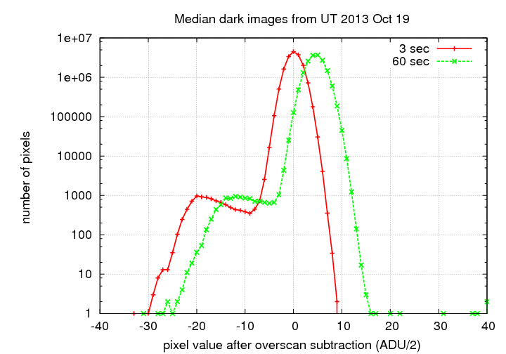
The long images have a typical pixel value which is larger than that of the short images; that makes sense. Based on these histograms, we could conclude that the dark current is roughly 5 (ADU/2) = 10 ADU over the course of 57 seconds. With a gain factor of about 1.3 electrons per ADU, that corresponds to a dark current rate of 0.23 electrons per pixel per second. This is considerably higher than the value of about 0.03 electrons per pixel per second derived in Tech Note 2.
I used the twilight sky R-band images to create a master flatfield, again with a pixel-by-pixel median algorithm. The result is shown below -- click to see a larger version.
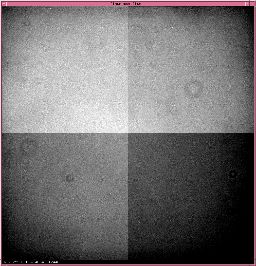
The intensity of pixels in the corners is roughly ten percent lower than the intensity near the center. There are very large dust donuts and medium-sized dust donuts, likely due to dust on the filter and dust on the camera window, respectively.
The MASTER OT field is at relatively low galactic latitude, b = 10 degrees. It has many stars with a range of magnitudes across the entire image. The FWHM is roughly 3.0 pixels = 1.3 arcseconds. The stellar images appear uniform across the image to the eye, but if one plots the FWHM as a function of row and column position, one can see a slight trend with rows:
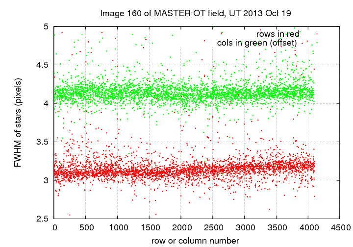
Since the large row numbers correspond to North, it appears that there may be a slight increase in FWHM towards the North end of the camera. However, the change is small: only 0.3 pixels = 0.13 arcsec from center to edge.
Inhomogeneous ensemble photometry of roughly 3000 stars in a set of 10 consecutive images yields an empirical measure of the precision of magnitude measurements. The basic idea is to assume that most stars are constant in luminosity, so changes in their apparent brightness are due to clouds, shutter issues, or other systematic effects.
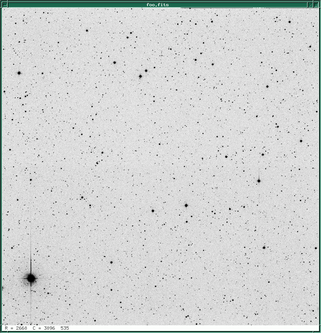
I analyzed 10 consecutive images, each 60 seconds long in R-band, of the field of MASTER OT J061335.30+395714.7. The field is at a galactic latitude of about 10 degrees, so there are plenty of stars. The image below has North up, East to the left. The variable star is near the bottom-right corner.
Each image is given a "magnitude offset" or "image adjustment" which brings its raw instrumental magnitudes as close as possible to their overall mean levels throughout the sequence. For this field, the offsets were several hundredths of a magnitude = several percent:
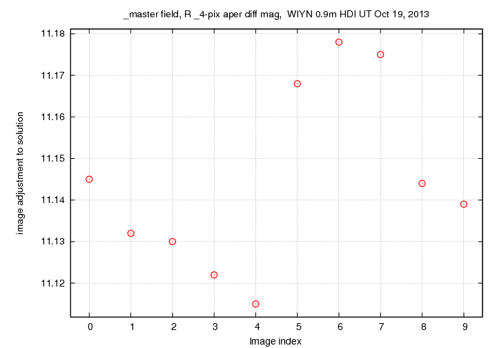
This suggests that the night was not photometric. The airmass of the exposures decreased during the sequence from 1.444 to 1.374, according to the TCS, so on a perfectly clear night, we should see the image adjustment decrease gradually.
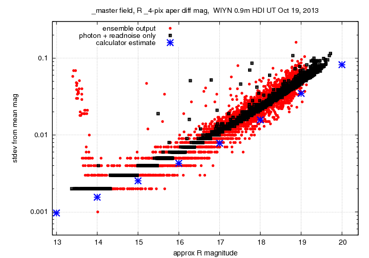
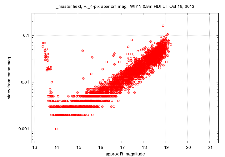
The ensemble analysis provides a measure the scatter of each star's magnitudes from its overall mean value. The graph below shows the expected and very typical pattern: large scatter for faint stars, small scatter for bright stars, and an increase at the very bright end for saturated stars. The horizontal scale shows very approximate R-band magnitudes, based on a zero-point calculation using just three stars.
We can compare these uncertainties to those which one would expect due to photon noise (based on the number of counts detected for each star) and readout noise. In the graph below, the expected uncertainties are shown in black. The good agreement between red and black symbols indicates that our simple noise model is a good one, and that there are no major additional source of noise. The blue symbols show predictions based on the WIYN 0.9-m signal-to-noise calculator. Those predictions are slightly optimistic, but only by a few tenths of a magnitude.