Contents:
This report describes my attempt to create a toy pipeline to reduce data from the Tomoe camera. The pipeline is not robust, nor is it well documented and easy to share. It's simply a set of tools, roughly placed into the appropriate sequence for turning raw Tomoe data into something like astrometrically and photometrically calibrated starlists.
The data I used to test this pipeline were taken from the "composite" FITS files
which cover a span of about 27 minutes during the night of Apr 11, 2016. The field is centered near (RA = 196.5 = 13:06:00, Dec = -16.20 = -16:12).
The pipeline uses a set of programs taken from
The various pieces are prepared and connected using a set of Perl scripts.
The pipeline is designed to work on one "composite" FITS file at a time. A "composite" file contains 360 individual images, stuck together to create a 3-dimensional data cube. After the pipeline has processed one "composite" file completely, it can process another. The results will not be combined automatically (at this point).
The stages of the pipeline are:
This document will describe very briefly each stage below. Note that "ensemble output" only includes objects which were detected in all, or nearly all, images; thus, a second round of calibration is required to give a position and magnitude to EVERY object which was detected, even if it appeared in only a single image.
The result is a set of magnitude offsets between the images, a set of mean magnitudes for the stars, and individual measurements for each star in each image.
The choice of V-band is arbitrary. We can pick a different choice as desired.
In order to calibrate them, a second round of astrometry is performed for one image at a time, including all the objects detected in it. The procedure is the same as that described above for the ensemble.
In order to calibrate them, a second round of photometry is performed for one image at a time, including all the objects detected in it. The procedure is the same as that described above for the ensemble.
I made no attempt to optimize the pipeline code. For example, during the astrometric calibration, the pipeline requests as sub-set of the UCAC4 catalog from the Vizier service to match the stars in each image. That request is sent for every one of the 360 images in a composite FITS file -- even though the images cover the same region of the sky.
I ran the pipeline on my MacBook Pro laptop, which is a 13-inch, Late 2011 model, with 4 GB RAM, 2.4 GHz Intel Core i5. The pipeline does not attempt any multi-threading.
Execution times varied slightly, but were typically 35-40 minutes per composite FITS file. Since a composite file contains 360 images, each with 0.5-sec exposure time, it covers a duration of about 3 minutes of real-world time.
The pipeline thus runs approximately 10 times too slowly to keep up with the data in real time, at least on my machine.
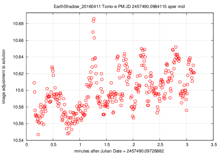
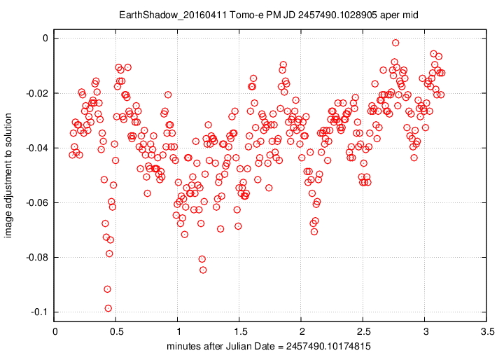
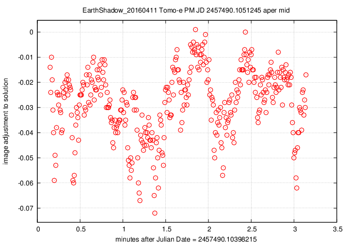
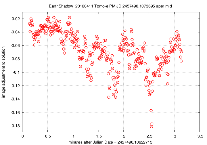
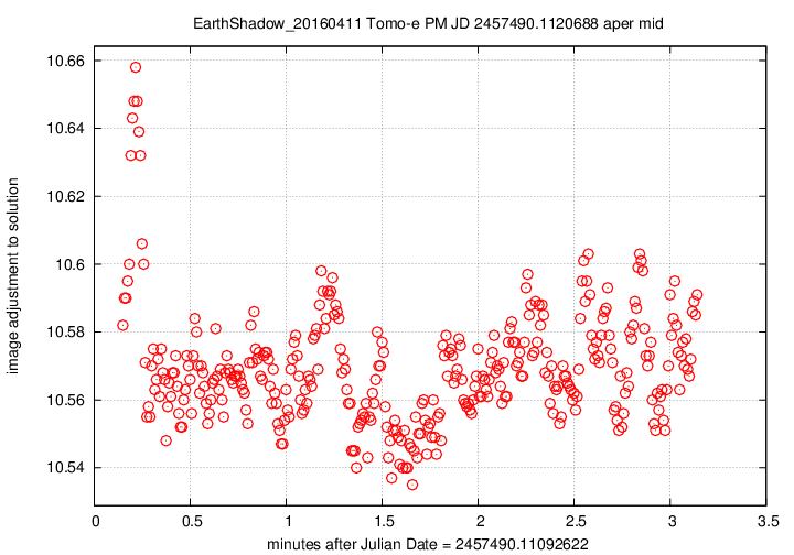
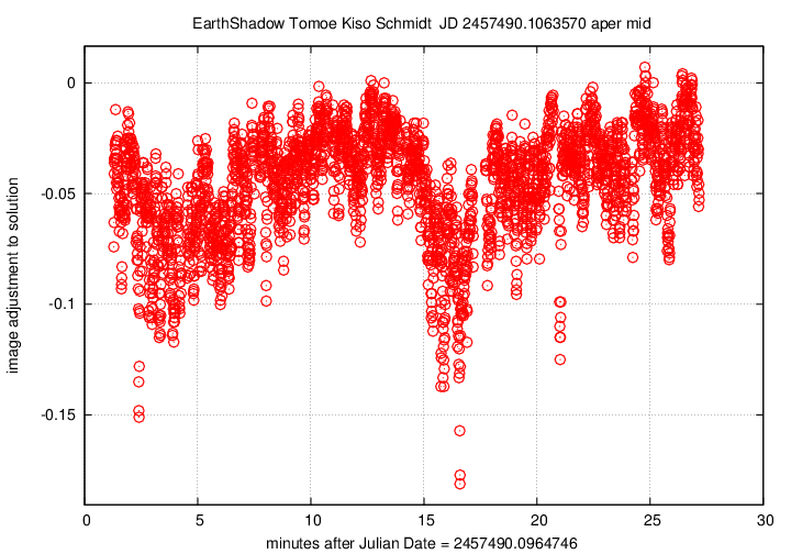
Let me begin with two graphs which show aspects of the data over the entire 26-minute span of time covered by the 8 composite FITS files.
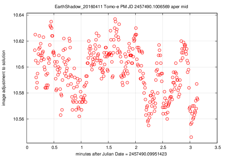
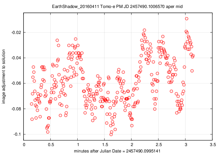
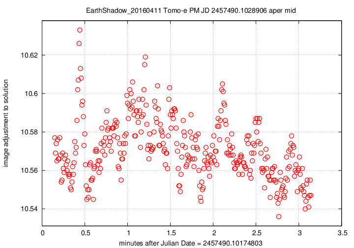
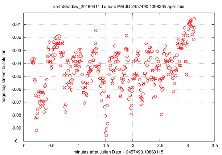
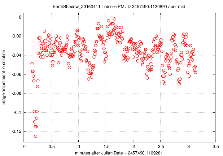
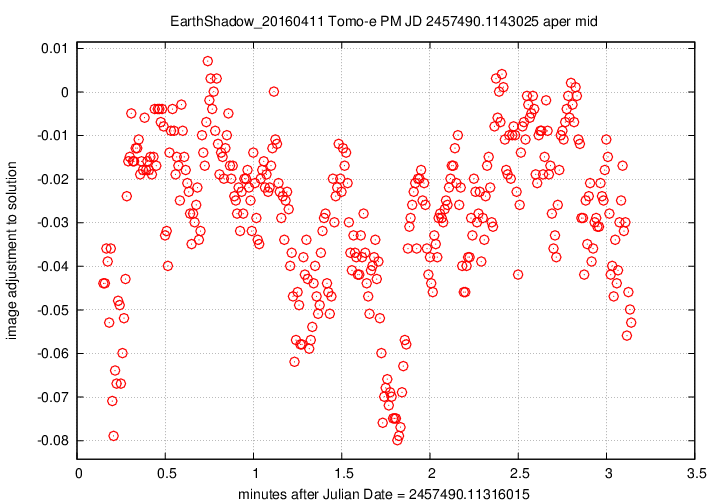
First, the offset in magnitudes between the UCAC4 V-band values for stars and their instrumental values, in the sense
(V-band magnitude) = (instrumental magnitude) + offset
We see slow, rolling variations over timescales of tens of minutes, together with quick variations on timescales of tens of seconds. The maximum variation is just 0.15 magnitudes, and the typical changes are only about +/- 0.03 magnitudes.
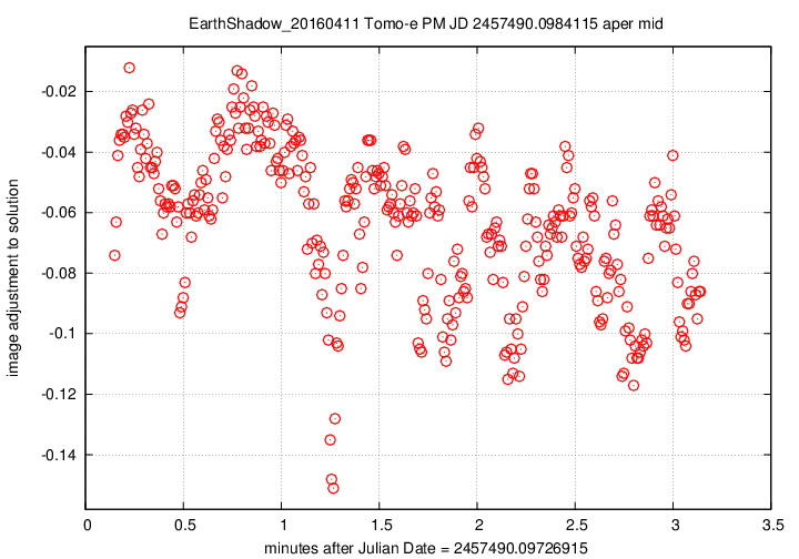
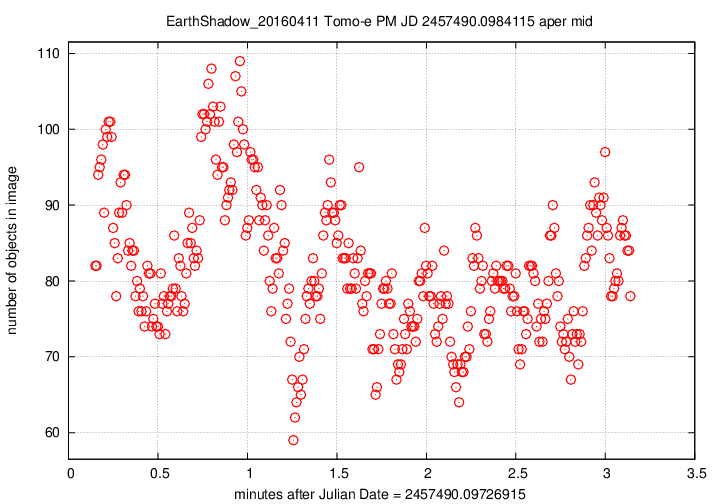
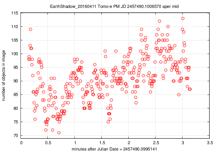
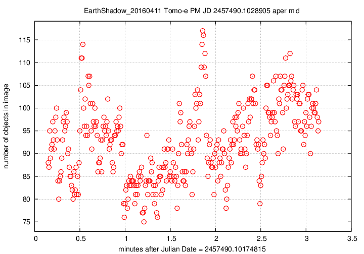
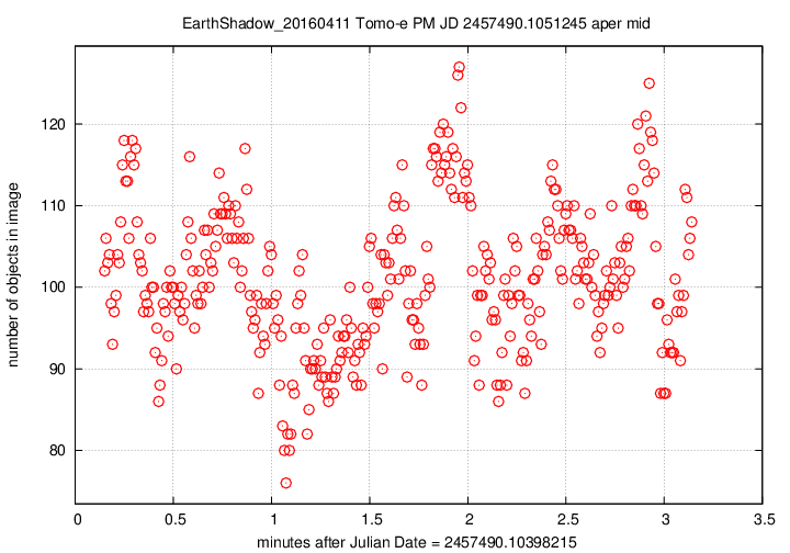
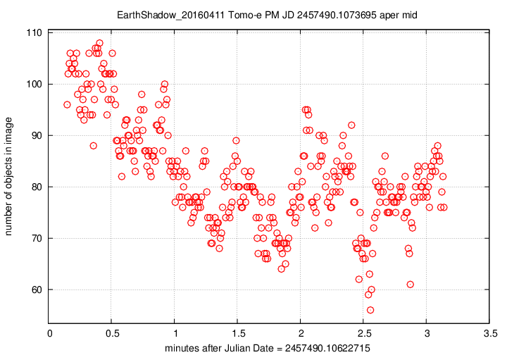
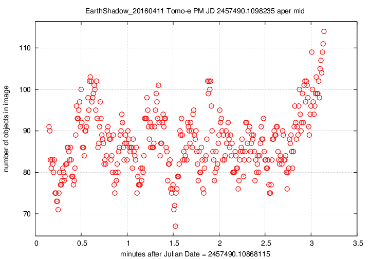
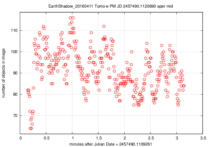
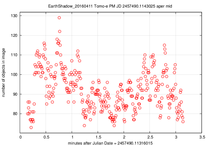
Next, the number of objects detected per image over this observing run.

The pattern is a mirror image of the magnitude value, which makes perfect sense: when clouds pass overhead, the magnitude offset changes, and many faint stars disappear. The changes here are quite large, up to 30% or 40% of the number of stars seen in the best images. This indicates that a large fraction of the objects are close to the plate limit --- again, no surprise.
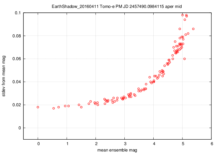
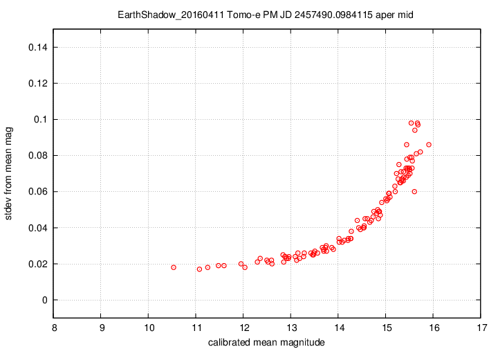
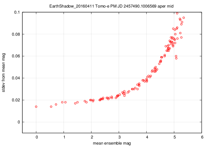
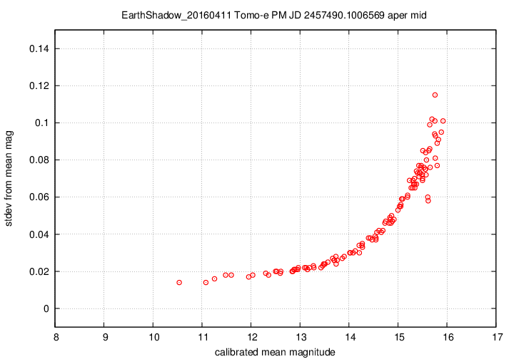
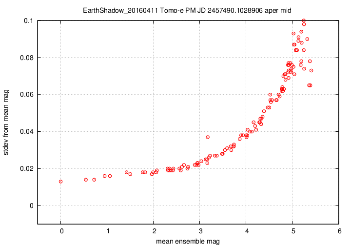
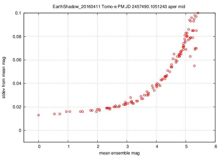
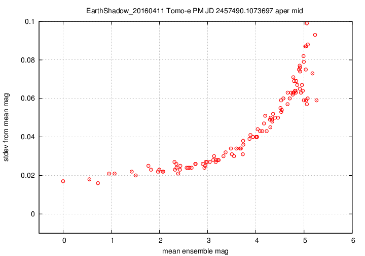
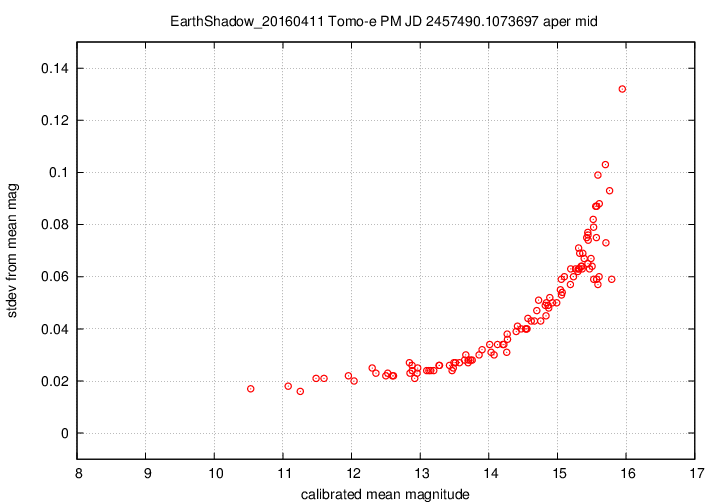
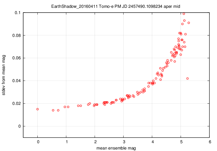
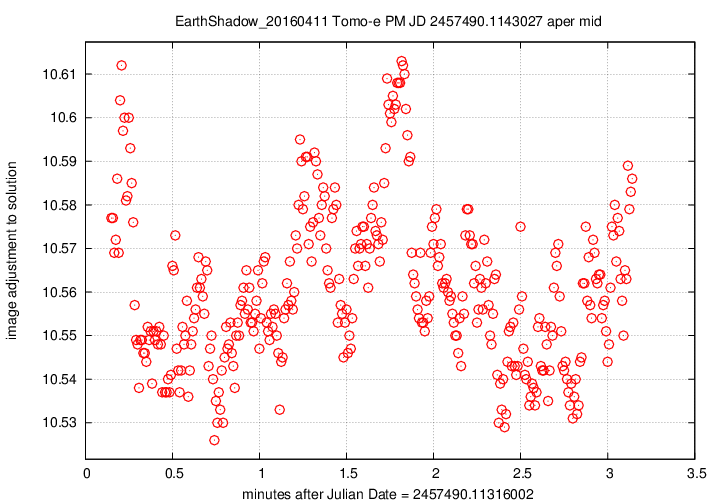
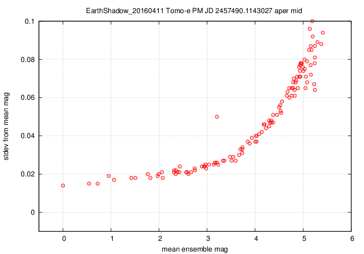
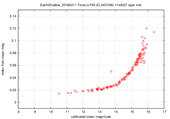
I don't have a single graph showing sigma-vs-mag for the entire dataset, but I'll place a graph showing this relationship for a single composite file (3-minute stretch of data):
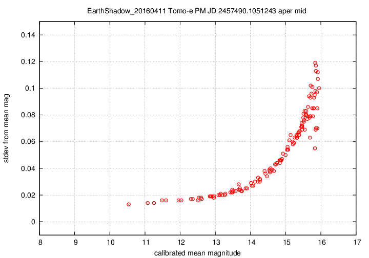
This graph shows the relationship for the "middle-sized" aperture: a circle with radius 8 pixels. The floor of the scatter is about 0.017 mag, somewhat higher than one might expect from simple signal-to-noise and scintillation calculations.
My plans for the future are to extend this work in the obvious directions.
This will be easy to do with the current results.
This will not be so easy to do. I have some ideas for efficient means of looking through the .ast files, which contain calibrated measures of every detected object, but I'm not sure which will work best for finding, say, "objects which appear in at least 3 but no more than 10 images."
Of course, I welcome suggestions for the direction I should take.