The Tomo-e Gozen Northern Sky Variable Survey contains many measurements of objects since 2018. This work examines measurements made between March 9, 2019, and May 31, 2023, in a region of the sky covering roughly 100 square degrees. Earlier pipelines have cleaned and processed the images, created catalogs of stars, performed aperture photometry, and calibrated that photometry against the Gaia catalog. I break this calibrated data into small subsets and apply inhomogeneous ensemble photometry in order to examine the actual uncertainties in the photometric values. I find that the photometric uncertainties listed in the source_stack table are underestimates, quite significantly at the bright end and slightly so at faint end.
What is "inhomogeneous ensemble photometry?" The term goes back at least as far as 1992, when R. Kent Honeycutt wrote his classic paper describing it.
The basic idea is that when one compares measurements of stars made on different nights, one may encounter somewhat large differences in the zero-point calibration from one night to the next; but that the inter-star differences within each night may be very stable. If one simply combines all the measurements without making any adjustments, the night-to-night variations may overwhelm any small intrinsic changes which appear clearly within each individual night.
The solution is then to determine first the night-to-night variations in zero-point, make corrections for them, and then to search for any intrinsic variation; but these night-to-night corrections might lead to somewhat different relative values for stars in the field, which would then require a second round of (smaller) zero-point adjustments ... which would lead to another somewhat (less) different set of relative values, and so on. One could pursue the goal iteratively, but Honeycutt showed how to use matrix operations to find a solution in a single (complicated) step.
I have implemented a version of this method
and used it profitably for many years to measure the light curves of supernovae, eclipsing binary stars, and other variable sources.
The Tomo-e Gozen Northern Sky Variability Survey has already performed photometric calibration for all its measurements. The algorithm runs as follows, in a very simplified form:
By subtracting one of the zero-point offsets from the instrumental magnitudes, one can calculate a calibrated magnitude for Tomo-e measurements. The source_stack table within the Tomo-e database contains several calibrated magnitudes for each detected objects, based on the slightly different recipes for the "synthetic" magnitudes.
For the purposes of this study, I chose to focus on the following quantities in the source_stack tables:
Now, since the measurements made on each exposure, in each chip, were calibrated individually, there should in theory be no zero-point differences between measurements made on different nights. In other words, if we were to compare the measurements of a set of ten constant stars on a single chip from one night to the next night, we should expect to see small, random changes in magnitude; the changes in each star should be uncorrelated. We should NOT expect to see that all the stars appear a bit brighter on the second night.
That's the idea, anyway. This study carries out a comparison of such night-to-night variations, to see if the theory holds. If not, if night-to-night (or exposure-to-exposure) systematic variations still exist, it might be possible to correct for them and so to improve the quality of the photometry of the stars.
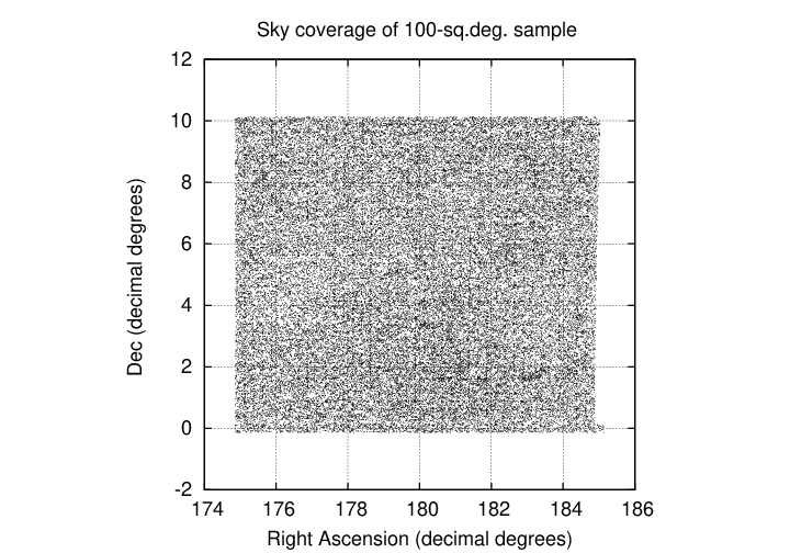
In order to test some ideas, I chose a dataset which is only a small fraction of the total available in the source_stack table. I picked a region of roughly 100 square degrees, within the boundaries (in decimal degrees)
The measurements included here cover the timespan from 2019 March 9 (MJD 58551) to 2023 May 31 (MJD 60095). The distribution of data with time can be seen in the graph below; the meaning of the vertical axis is not important, but it does act to spread out the symbols and make it easier to judge the number of measurements on each night.
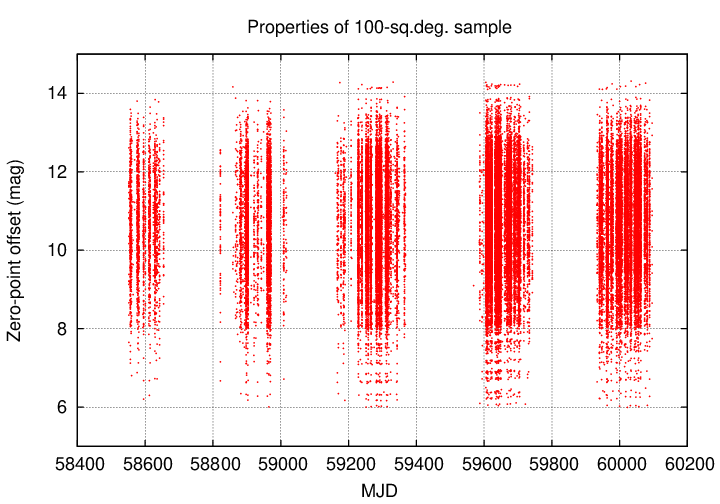
The figure shows several features:
The original measurements are based on chips (= sensors = detectors): images recorded on a single sensor, during one exposure of duration 0.5 seconds. These images were then stacked in groups of 12, before Aug 14, 2020 (= MJD 59076), yielding an effective exposure time of 6 seconds; or in groups of 18, after Aug 14, 2020, yielding an effective exposure time of 9 seconds. These stacked images were cleaned in the usual manner, with dark-subtraction and flat-fielding. the SExtractor program then identified stars and measured aperture photometry using a number of different apertures. My choice of the "magauto_zmr" value is based on an aperture which depends on properties of each image, using the Kron radius as a guide. The instrumental magnitudes were calibrated for each stacked chip individually, as described earlier, and the resulting calibrated Tomo-e magnitudes were inserted into the source_stack table of the database.
My work began with these calibrated magnitudes.
Now, if the entire measurement and calibration process had been perfect, then there would be no need for any further work. If one chose a particular region of the sky, and examined the repeated measurements of some set of stars over a period of time, one ought to see
Therefore, if we were to create an ensemble for these stars in this small region of the sky, and perform the standard inhomogeneous ensemble procedure, we ought to find NO epoch-to-epoch changes in the zeropoint; or, more precisely, we ought to see only tiny, random variations due to the small random variations in the measured magnitudes of the stars due to photon and sky noise only. Since the ensemble procedure combines measurements of all the stars, these small random changes would be made even smaller through a sort of averaging.
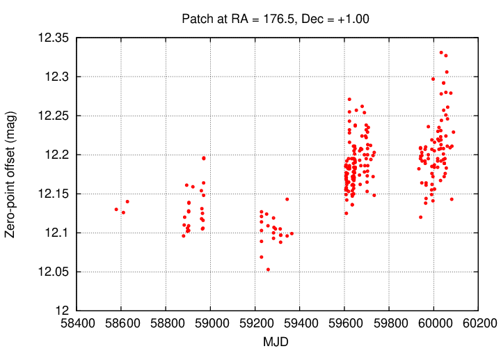
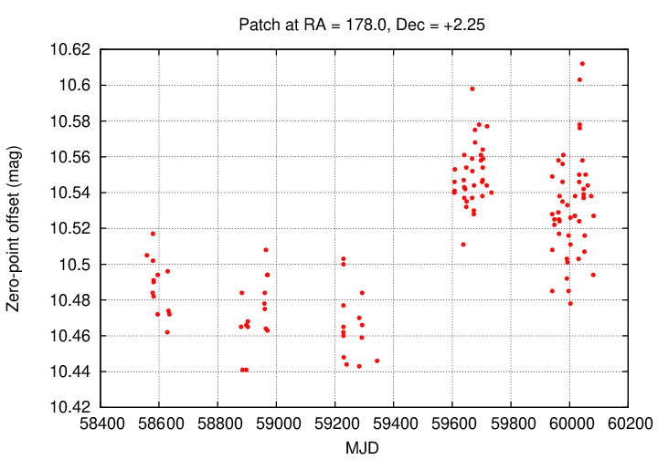
However, when I actually did carry out this ensemble analysis using the source_stack measurements as input, I found significant changes in the zero-point from one epoch to the next. Below is an example for one randomly chosen patch, centered at (RA = 176.5, Dec = +1.00).
Zooming in to one small stretch of time, we can see what happens within the course of single nights (often the same field was observed 3 or 4 time during a night).
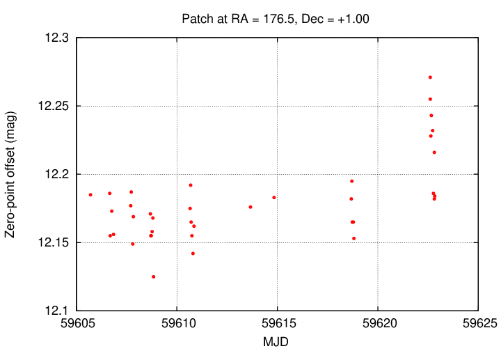
What do we see?
This one field may not be completely representative of the entire region of one hundred square degrees, but it shows that at least some of the data does suffer from small, but (in some cases) significant systematic errors. By running ensemble photometry, we can
Point (b) is an important limitation on this work. The ensemble analysis will place all the stars within each small patch onto a consistent photometric scale, which can be shifted so that the mean magnitudes of the stars are approximately the same afterwards. However, the solutions for each small patch are derived independently, and so there may remain small zero-point offsets between the solutions in patch A versus patch B and patch C, and so on. In other words, this procedure may introduce its own (small) zero-point offsets between all the patches in the region.
In short, the result will be photometry which is definitely more PRECISE within each patch -- and so good for some purposes -- but which _may_ be less ACCURATE across the entire region -- which may cause problems for some types of analysis.
Let me describe briefly now how I processed this dataset. I encountered two minor problems, both of which I was able to solve; one of them could be an important piece of information that users of source_stack should know.
First, I divided the 10-by-10-degree region into small areas which I will call patches. Each patch is 0.25-by-0.25 degrees with boundaries parallel to the RA and Dec axes. After calculating the values of the minimum and maximum RA and Dec values for the patch, I ran the following query to select all observations of objects within a patch from the Tomo-e database:
 SELECT \"rawId\", \"expId\", \"detId\",
        ra, dec, magauto_zmr, magautoerr, fwhm, classstar
   FROM source_stack
   WHERE q3c_poly_query(ra, dec,
         ARRAY [ $min_ra, $min_dec, $min_ra, $max_dec,
                 $max_ra, $max_dec, $max_ra, $min_dec ] )
   ORDER BY \"rawId\"
For such small areas on the sky, the query does not take much time; in most cases, about 1 second. There were a total of 1641 patches.
Next, I used the expId value for each entry to look up the Modified Julian Date of the measurement; one can find the relationship in the rawId table. The equation for MJD is
MJD = Julian Date - 2,400,000.5
I then split all the measurements into individual groups by the date of observation, so that all measurements of stars made in the same exposure were collected together. This is necessary for the ensemble analysis.
At this point, I ran the ensemble analysis code, which works in two steps.
In this step, interesting parameters are
              - matching radius of 3 arcseconds
              - images must have at least 40(*) stars to be included
              - stars must appear in at least 30 images to be included
Typically, this step took about 5 seconds per patch.
(*)One of the problems that occured rarely in the processing involved regions of the sky with few stars. In 4 out of 1641 patches, I had to decrease the minimum number of stars in an image to 30. Note that 40 stars in a patch corresponds to a stellar density of (40*16) = 640 stars per square degree.
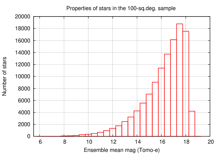
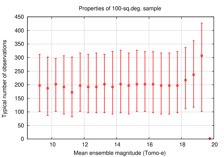
The two graphs below show some overall properties of this selection of stars. A rough estimate of the limiting magnitude is around mag ~ 17, and each star typically is measured between 100 and 300 times.
I discovered one somewhat significant problem with the source_stack dataset during this matching procedure. In a small number of patches -- 10 out of 1641 -- the initial attempt at matching up stars failed due to a large number of bogus "stars" recorded in some of the exposures. To illustrate the effect, look at the figure below. It shows the positions of objects from the database in one particular patch at four different epochs; each epoch is shown with a different symbol. The red symbols come from an ordinary exposure: stars are scattered evenly all over the patch. But objects taken from three other exposures, shown in dark blue, cyan, and green, reveal the problem: although some of the objects in these exposures are real stars, appearing at the same locations as those in the ordinary exposure, each shows a long vertical line of "objects". These are clearly bogus detections; my guess is that some sort of column defect was not masked properly.
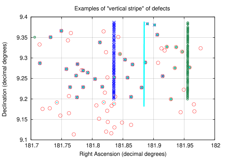
In some patches, many of the exposures suffered from this problem. In some cases, 10 or 20 out of 200 exposures showed these vertical stripes of bogus objects. The implication is that some fraction of the objects in the source_stack table may be defects, rather than real celestial objects.
Typically, this step took about 3 seconds per patch.
The results of this calculation are a set of relative magnitudes for the stars; the zero-point is arbitrary. In order to place the magnitudes back onto the same scale as found in source_stack, I used the following method:
The results of this step in the analysis are three-fold: a list of the zero-point adjustments which need to be made to each patch, the mean magnitudes of each star in the patch, and the light curve of each star after the zero-point corrections have been made. The graph below shows one example of the zero-point shifts for one particular patch:
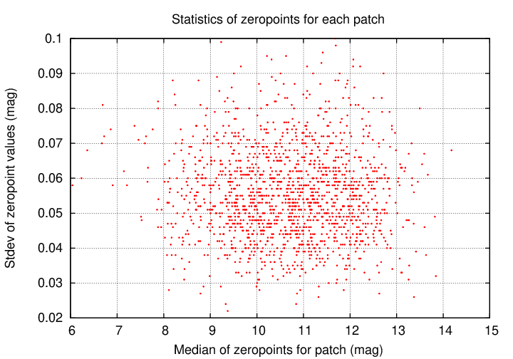
If we compute the average value of the zero-point offsets for each patch individually, and then calculate the standard deviation around that mean, we can see the typical size of these epoch-to-epoch variations for each patch. The graph below shows these standard deviations for all the patches. The important quantity is shown on the vertical axis; the quantity on the horizontal axis is something of an artefact of the processing.
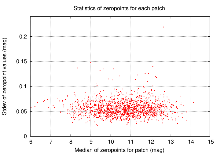
A closeup on the bulk of the values is shown below. Note that the typical size of these variations is 0.05 to 0.06 mag. Without making these corrections, photometry of individual objects at levels of 0.02 or 0.03 mag will be unusual.
Overall, the ensemble analysis for 1641 patches covering 100 square degrees took a total of 6.5 hours on the machine 'shinohara1'. Some statistics on the output:
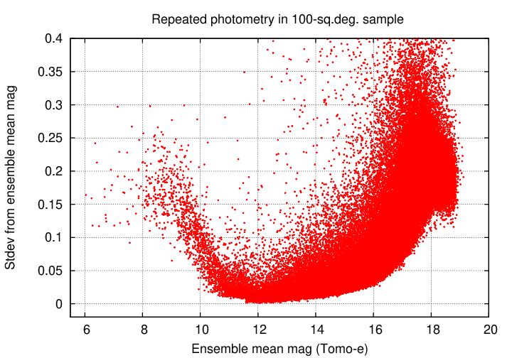
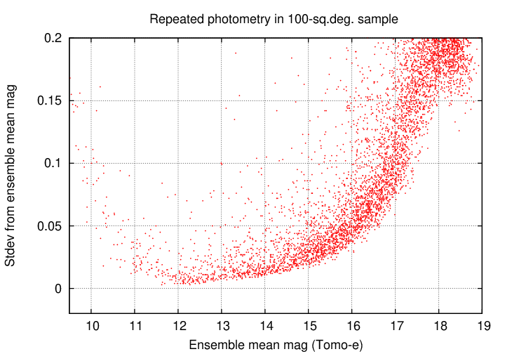
One of the most fundamental results from any sky survey is its photometric precision: what is the scatter in measurements of a "constant" star? Let's examine the results of this ensemble analysis and compare it to the properties of the uncorrected source_stack data.
First, this graph shows the standard deviation from the mean value for all stars in the region (aside from some which fall off the top of the graph). Note the "rooster tail" for very bright stars: at magnitudes less than 11, the scatter increases with brightness, due to saturation.
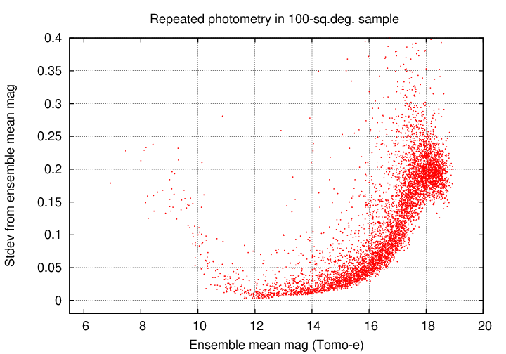
We can see some features more clearly if we plot only every twentieth datum. Note that something strange happens for the very faintest stars, around mag 18; the standard deviation SHOULD continue to increase, but it reaches a plateau. I am not sure what causes this to happen, but it indicates that measurements of the very faintest stars are somewhat suspect (which is not any surprise).
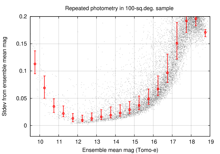
Let's zoom in, so that we focus on stars with small standard deviations.
I placed stars into bins by magnitude and computed the quartiles within each bin. The graph below shows the median value as a circular symbol, with errorbars running from 25th to 75th percentile. Comparing the symbols to the measurements, it appears that the 25th percentile is a better estimate of the floor of this distribution than the median (due to the main outliers in the positive direction only).
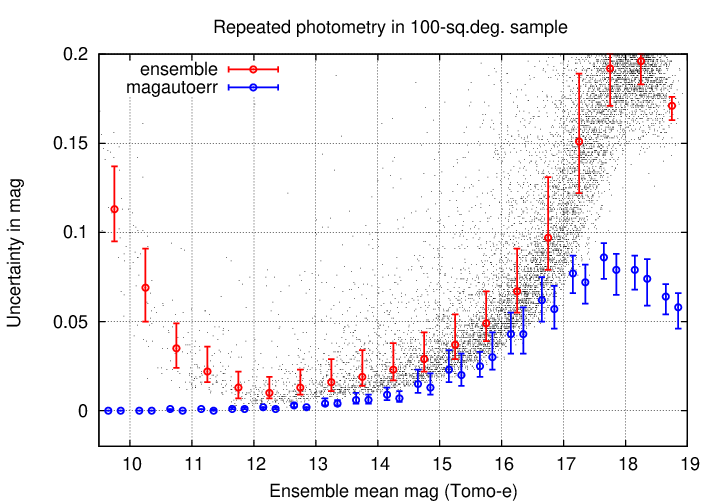
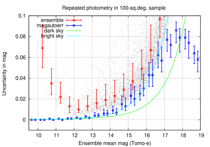
The source_stack database provides estimates of the uncertainty for each measurement, based on a combination of SExtractor's output and a contribution from the calibration step. As noted above, I chose the magautoerr column from the database as an indicator of the uncertainty in each magnitude. The graph below shows the median values of binned "magautoerr" values; for technical reasons, I selected two random subsamples of tens of thousands of measurements for this comparison, rather than using the millions in the database.
Two facts are clear:
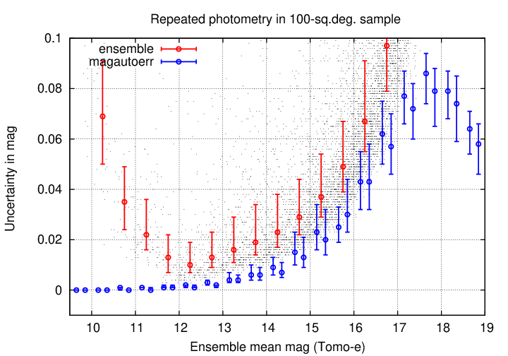
Zooming in further, we see that the magautoerr values do come reasonably close to the post-correction scatter for stars of middling brightness (15 < mag < 17).
I used a CCD signal-to-noise calculator to compute theoretical values for the uncertainty in Tomo-e measurements, using a set of reasonable assumptions:
In the figure below, the cyan curve shows the uncertainty for photometry in the case of a "bright sky", mag 19.0 per square arcsecond; the green curve shows the results for a "dark sky", mag 21.0 per square arcsecond.
Note that the magautoerr estimates are close to those computed in this theoretical manner for the "bright sky" case. This is not too surprising, as SExtractor uses similar methods based on the statistics of electrons in the image. The fact that both magautoerr and my calculator yield UNDER-estimates of the actual scatter -- even after correcting for zero-point offsets -- indicates that there are significant sources of error in the data collection and analysis that have not been identified and corrected.
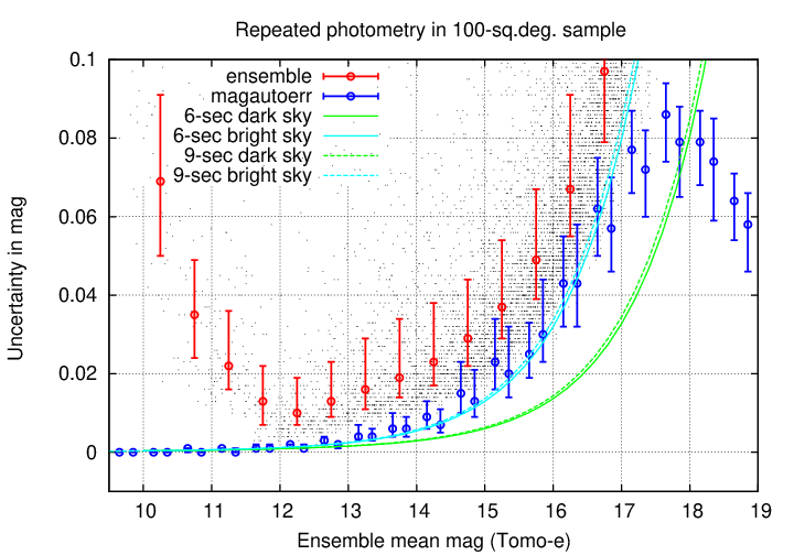
The graph below shows the theoretical results for exposure times of both 6 seconds and 9 seconds; the difference is negligible. That's good, as the source_stack table contains a mixture of measurements acquired with both exposure times: 6 seconds before Aug 14, 2020, and 9 seconds after that time.
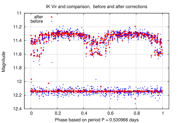
To illustrate the difference between the original source_stack photometry and the output of the ensemble procedure, I have chosen two variable stars in the survey area: IK Vir and V0672 Vir. I chose these two stars because they have relatively small amplitudes of variation, and so will show clearly any improvements made by the ensemble procedure.
IK Vir is classified as an EA-type eclipsing binary. Its period is not listed in the GCVS, so I searched for it myself. The best value appears to be around 0.530966 days, but no value seems to give a light curve with clean dips at primary and secondary max; my guess is that the period is changing relatively rapidly, and these measurements over 5 years show the effects.
In the graph below, IK Vir is shown near the top of the panel, and a nearby comparison star near the bottom of the panel. Magnitudes taken from source_stack are shown in blue, and those produced by the ensemble analysis in red.
A second example is given by V0672 Vir, an EW (W UMa) type eclipsing binary. In this case, the GCVS provided a period of P = 0.361755 days; however, I found that a slightly larger value, P = 0.361758, produced a nicer light curve. In this figure, I've shifted the measurements of the comparison star downward by 0.1 mag for clarity.
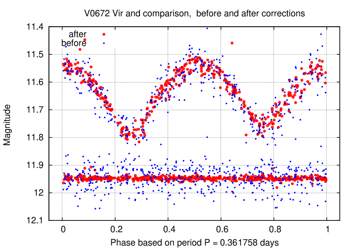
It seems clear from these two examples that the analysis of variable stars, at least, will benefit from the increased precision provided by ensemble analysis.