This document describes tests of the Tomoe pipeline's efficiency in detecting artificial stars which have been added to real images.
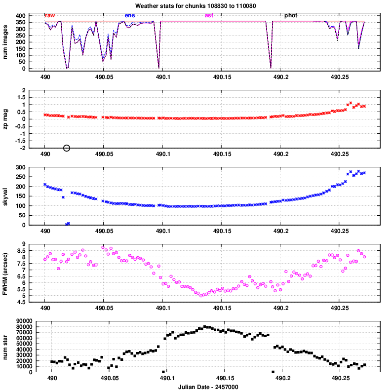
The efficiency of any star-finding algorithm can vary depending on the nature of the images it is given. In order to check the Tomoe pipeline under a reasonable range of conditions, I chose as the dataset a portion of one night, during which the seeing changed significantly. The night of 2016 April 11 featured poor seeing at the start and end, but decent seeing in the middle. Below is the "weather report" for chip 0 of this night; see Tech Note 7 for more details.
I used images from chip 0 only; these have very slightly worse properties, on average, than images from chips closer to the center of the field of view.
I selected the following subset of this night for the artificial star tests:
                  Start                       End
   ----------------------------------------------------------

    chunk        10910                       10955

    JD           2457490.05164               2457490.15577

   ----------------------------------------------------------
The FWHM of the PSF ranged from 7.5 to 4.2 arcseconds, improving throughout this interval. The typical number of objects detected in each image ranged from roughly 50 to 250, depending on the seeing.
The first series of tests involved adding artificial stars to all the images within a chunk, running the pipeline, then checking to see how many times (out of approx 360) each artificial star was detected. For the most part, this should yield the same results as the tests with real stars shown in Tech Note 002 , but let us see if that expectation is met.
I used the XVista command pstar to add stars to the real Tomoe images. Each star was modelled as a simple, circular Gaussian profile. The FWHM of the Gaussian was set to the average FWHM for real stars in the chunk, and photon noise (but not other sources of noise) were included in the generation of each artificial star.
In order to prevent a large number of collisions and overlap between the artificial stars and real stars, I added only 10 artificial stars to each image. Thus, in the 46 chunks of data used in this test, there were a total of 460 artificial stars.
The procedure was as follows:
For simplicity, I assigned a fixed (row, col) position to each artificial star. During the course of a chunk of 360 consecutive images, real stars would wander slightly in (row, col) position, due (mostly?) to atmospheric motion and (less?) to imperfect telescope tracking. I did not attempt to follow this motion with the artificial stars, so they appeared to move slightly relative to the real stars. The amplitude of these artificial drifts can be seen in the graph below.
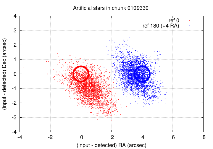
Each cloud of points shows the difference between the derived (RA, Dec) position of an artificial star in one "reference" image within the chunk, and the derived (RA, Dec) position derived for that star in other images within the chunk. The red symbols mark the results when I chose the very first image in a chunk to convert the artificial (row, col) position to (RA, Dec). As you can see, most of the image motion was in one direction, carrying the artificial star to the south and east. In order to link together all detections of an artificial star to the reference, one might need to use a matching radius of about 4 pixels in this case.
After I noticed this rather pronounced image motion, I chose to use the middle image in chunk, number 180 out of 360, as the "reference" for converting the generated (row, col) position into (RA, Dec). Note that with this convention, the cloud of derived positions for the artificial stars is more nearly centered on the reference location; that means that one can use a smaller matching radius and still link together all detections.
In the end, I adopted a matching radius of 4.0 arcseconds.
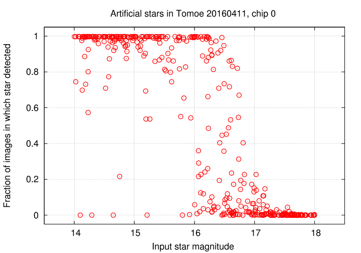
So, how frequently did the pipeline detect an artificial star? At first blush, it appears that many bright stars were missed in 10 or 20 percent of their images.
However, if we separate the results into those which were measured during good seeing, defined as "FWHM < 5.5 arcseconds", and those which were obtained under poor seeing, the situation becomes more clear:
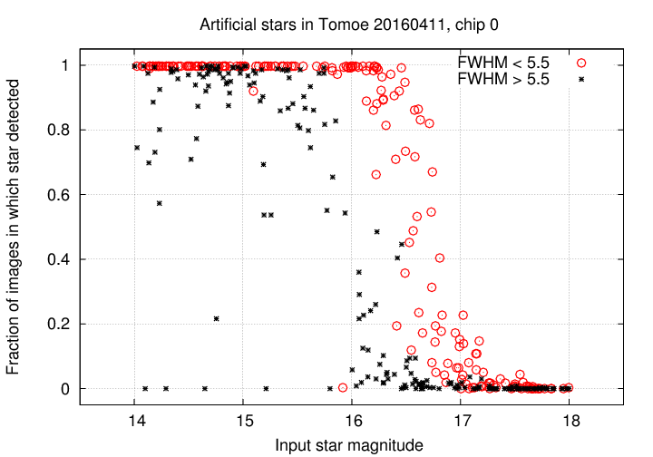
When conditions are good, bright objects are detected in all or very nearly all images; the completeness falls to 50% at around magnitude V = 16.5. However, when the seeing is bad, even very bright stars may be missed in a signficant fraction (10% to 30%) of their images.
Only a small fraction of artificial stars fell close enough to the edges of the frame to lead to non-detection.
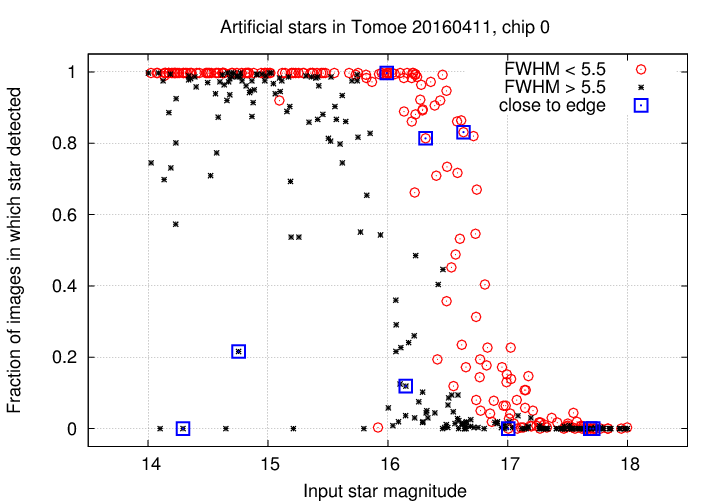
These results are similar to those described in Tech Note 002 , but provide additional information. Good.
The second series of tests involved adding artificial stars to SOME of the images within a chunk, running the pipeline, then checking to see if each added star was identified as a transient source. The procedure was the same as that described above, with the following exception: when generating an artificial star, in addition to quantities such as row, col, mag, each star was assigned a lifetime, first image, and last image.
In the simulations, I generated artificial stars with the following properties:
Starting images were chosen randomly from all those which would allow a star to complete its lifetime before the end of the chunk. In other words, each transient object in these simulations (unlike transient objects in the real sky) was guaranteed to appear only within the boundaries of a single chunk of images.
Note that the procedure which searched for transient objects used the same parameters as the code which was run on the real 2016 Tomoe data: an object was only accepted as a "transient" if it
Let's see what happened in practice.
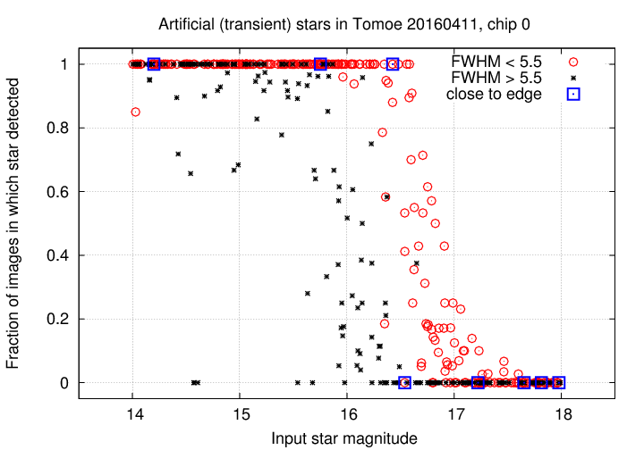
The graph below shows the fraction of all possible images in which a transient source was detected. The pattern is the same as that for constant sources: when the seeing is good, objects are found almost perfectly down to about mag 16.5; but when the seeing is bad, a substantial fraction of even bright stars are missed in some images.
But the real question is -- how often were the artificial objects correctly identified as "transient" sources? Of the 460 artificial objects, 315 should NOT have been classified as "transient", because they
That leaves (460 - 315) = 145 objects which SHOULD be detected and classified as "transient". The actual number identified by the classifying software was 111. Why were 34 objects not classified properly? The graph below offers an answer.
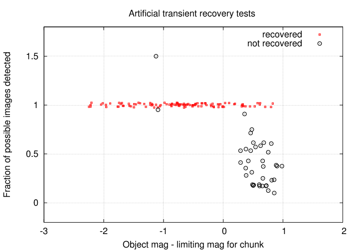
The horizontal axis has been changed to show the difference between the magnitude of an artificial star, and the limiting magnitude (at which 50% of real stars are detected) for the image. The message is clear:
    transient sources are identified almost perfectly
             as long as they are brighter than the limiting magnitude

    BUT

             are often missed when they are fainter than the limiting magnitude
The two bright objects which are not recovered properly have relatively benign explanations:
The conclusion I draw from these simulations is that, as long as we restrict the magnitude of possible transient objects to be no fainter than the limiting magnitude of a chunk, we can state with some confidence that the pipeline procedures will correctly identify 95% of all real transients.