Justin Rogers gathered some data from the SDSS for tests of photometry.
Attached is the data for 62 stars with r < 20 in a different field located at a right ascention of about 37.3 degrees (previous set was at 23.3). The objects have 18-32 matches in 63 different fields. I've also included the fiberMag's and their errors as "fu, fg, fr, fi, fz".
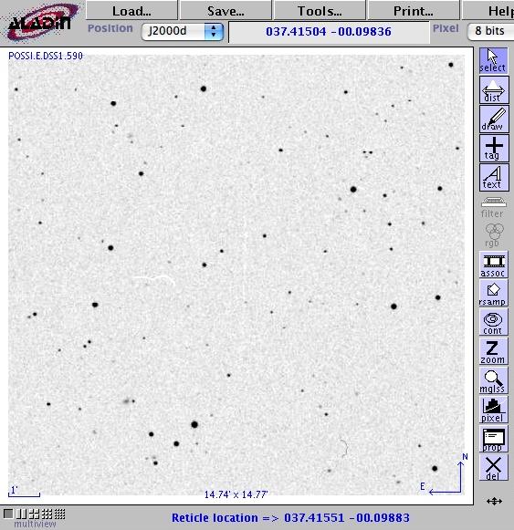
The stars fall within a box with rough limits 37.34 < RA < 37.51 and -0.21 < Dec < +0.01 The photometry comes from repeated scans of the celestial equator, some as part of the SDSS Supernova Survey. These scans were made over the past few years, with Julian Dates ranging from 2,451,075 (Sep 18, 1998) to 2,453,641 (Sep 27, 2005).
Here's a picture of the field, taken from the POSS-I plates, courtesy of Aladin.
I used my ensemble photometry package (with very minor modifications) to
My primary tool for gauging the quality of a solution was the scatter-versus-magnitude relationship: if the scatter of most of the stars is relatively small, then the solution is good. Since stars at the bright end might be saturated, I looked at them carefully, and marked as "variable" any which showed a scatter larger than expected; these "variable" objects are not used to determine the photometry solution, but do appear in the output.
I will show the results for each passband in a series of graphs below. Each displays scatter from the ensemble mean magnitude on the vertical axis, and the mean ensemble magnitude on the horizontal axis. Note that the brightest stars tend to show elevated scatter (in some cases too high to appear on on the graph); almost all of these are, I believe, due to saturation. I show on each graph the level corresponding to a scatter of 0.01 mag = 1 percent. There are black squares showing the estimated RMS for stars, based on theoretical calculations of the telescope and filter throughputs, etc. from Gunn et al., AJ 116, 3040 (1998).
I will provide two graphs for each passband: the first uses the PSF-fitting magnitudes in Justin's datafile, and the second the "fiber" (aperture) magnitudes. As you will see, the aperture magnitudes are better suited for our purpose, as one would expect.
Using PSF-fitting magnitudes:
Using "fiber" (aperture) magnitudes:
Using PSF-fitting magnitudes:
Using "fiber" (aperture) magnitudes:
Using PSF-fitting magnitudes:
Using "fiber" (aperture) magnitudes:
Using PSF-fitting magnitudes:
Using "fiber" (aperture) magnitudes:
Using PSF-fitting magnitudes:
Using "fiber" (aperture) magnitudes:
I provide below some of the output files from the ensemble solutions. The ".sig" files look like this:
     0 13.193  0.158  0    0.25     35.32486      7.03099
     1 11.360  0.073  0   -0.26     35.33325      6.72861
     2 12.190  0.078  0   -0.75     35.33335      7.18730
     3 13.695  0.137  0   -0.84     35.34351      6.66053
The columns in this file are
Below are files showing the full light curve of each star (well, actually, the values for all stars in a passband are gathered together in a single file). You can find the format of these files described in the ensemble package documentation; look at the section describing solvepht.out files.