On the night of May 20/21, 2018, from about midnight to dawn, I acquired a set of observations of the likely black-hole system MAXIJ1820+070, (also known as ASASSN-18ey ). Near the end of the run, condensation formed somewhere in the optical train (probably on the dewar window), ruining the last half hour or so of measurements.
This page also contains a section describing methods to remove the "vertical stripes."
The main setup was:
Notes from the night:
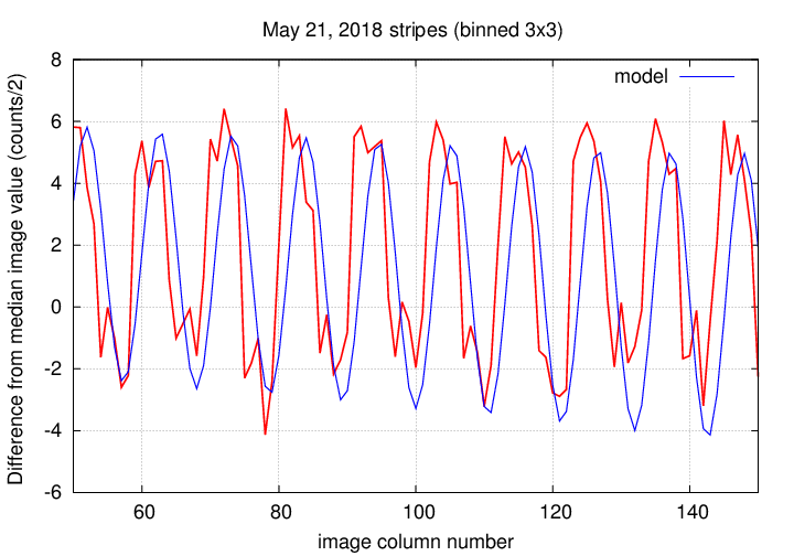
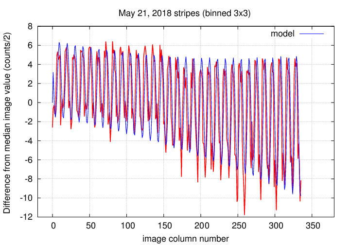
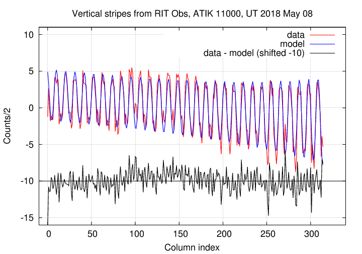
Tonight's stripes were modeled as follows:
                       2
        [         ( x ) ]       ( 2*pi*x      )   [             x    ]
 y(x) = [ 4 + 5.0*(---) ] * cos (------ + 1.4 ) + [ 2.5 - 6.0*(----) ]
        [         (400) ]       ( 10.666      )   [            400   ]
I see now that I didn't get the phase shift quite right. Oh, well.
This optical and X-ray and radio transient is likely a black hole accreting material at a higher-than-usual rate. It has been the subject of many observers over the past two weeks -- see the trail of telegrams that include
The object is located at
RA = 18:20:21.9 Dec = +07:11:07.3
A chart of the field is shown below. The size of the chart is about 22 by 18 arcminutes.

I've marked the location of several comparison stars, which also appear in light curves below. Stars C, D, and E are mentioned by the Tomoe Gozen team in ATel 11426, but all three are rather red, with (B-V) ranging from 1.14 to 1.37. Star B is one of the bluest nearby bright stars, with (B-V) = 0.52.
  star        UCAC4              B          V
----------------------------------------------------
   B       486-079513        12.975     12.454
   C       486-079608        13.968     12.830
   D       486-079523        14.637     13.272
   E       487-077858        14.637     13.272

----------------------------------------------------
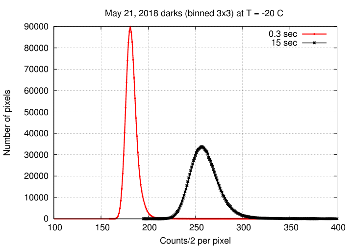
The dark current was ordinary.
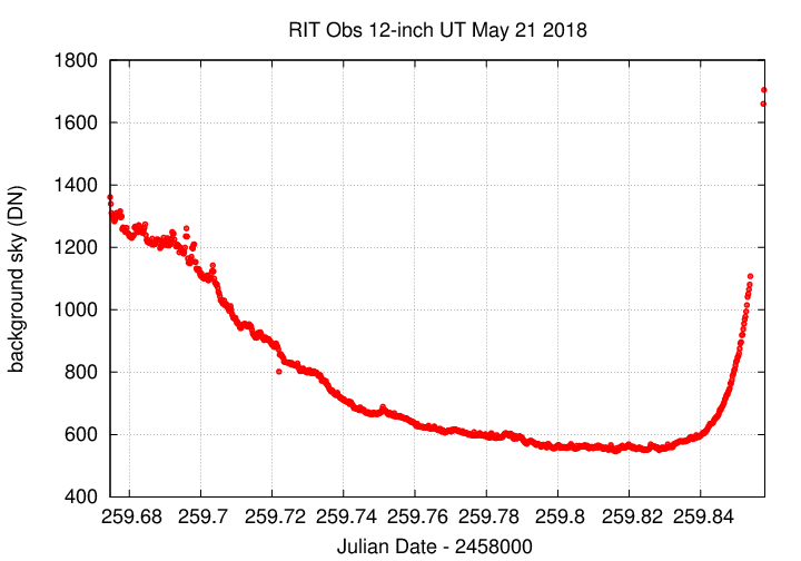
The sky value shows some light clouds early, then pretty much clear.
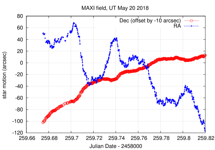
Here's a record of the telescope's drift. Guiding was turned off, and the telescope drifted quite a bit.
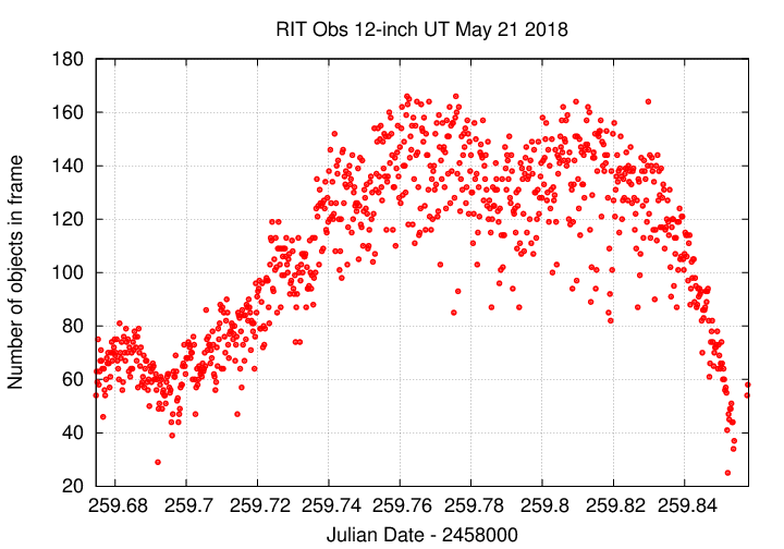
The number of objects detected took a sharp dive when the condensation appeared, around frame 730 = UT 07:40 = JD 259.8198. I discard all data after frame 729.
I used an aperture with radius 3.0 pixels.
Image adjustment factor shows some light clouds early.
![]()
Using aperture photometry with a radius of 3 pixels (binned 3x3, each pixel is 1.98 arcsec, so a radius of 5.9 arcsec), I measured the instrumental magnitudes of a number of reference stars and the target. Following the procedures outlined by Kent Honeycutt's article on inhomogeneous ensemble photometry, I used all stars available in each image to define a reference frame, and measured each star against this frame.
Sigma-vs-mag plots show that the floor was about 0.006 mag overall. The outlier around instrumental magnitude 2.3 is MAXI J1820+070. Note how much smaller its variations have become -- it used to tower over all the other measurements.
![]()
Here are light curves of the variable and the field stars. The bright star "A" was slightly saturated, so I marked it as "variable" in the ensemble.
![]()
I used the UCAC value for the V-band magnitude of star "B" = UCAC4 486-079513 to shift the ensemble magnitudes to the standard V-band scale -- but remember that these are UNFILTERED measurements.
Here's a closeup on the variable. I'll connect the dots to make its behavior a bit easier to see. Since I only started observing after the target had risen far above the horizon, there is none of the usual color-dependent extiction.
![]()
You can download my measurements below. A copy of the header of the file is shown to explain the format.
# Measurements of MAXIJ1820+070 made at RIT Obs, UT 2018 May 21,
#    in good conditions,
#    by Michael Richmond,
#    using Meade 12-inch LX200 and ATIK 11000.
# Exposures 15 seconds long, no filter.
# Tabulated times are midexposure (FITS header time - half exposure length)
#    and accurate only to +/- 1 second (??).
# 'mag' is a differential magnitude based on ensemble photometry
#    using a circular aperture of radius 3 pix = 5.9 arcseconds.
#    which has been shifted so UCAC4 486-079513 has mag=12.454
#    which is its V-band magnitude according to UCAC4.
#
# UT_day             JD            HJD        mag    uncert
May21.17481     2458259.67481  2458259.67888  13.101  0.013
May21.17521     2458259.67521  2458259.67928  13.078  0.014
May21.17563     2458259.67563  2458259.67970  13.112  0.013
Up to, and including, this night, the method I've used to remove the "vertical stripes" issue has involved several steps:
I even spent a fun day (really!) coding a program to do a very specific sort of optimization, in order to find the best-fit values of the parameters to the model.
The reason I chose to build a model was in order to avoid quantization effects. I thought that a smooth function of column position might be a more accurate representation of the real physical effect in the images. But -- is building the model really necessary? Does it really do a better job of removing the stripes than just using the master column vector itself?
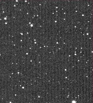
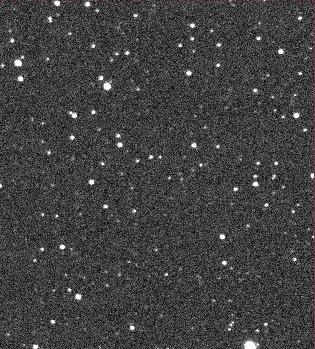
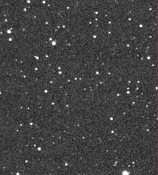
To answer this question, I picked 3 sample images from the night of UT 2018 May 08, each taken in good conditions:
I generated both a master column vector from hundreds of images on May 08, and then fit a model to that column vector. The model's form was pretty complicated:
                   x  3           2*pi*x
  y  =  [ A +  C*( - )  ]  * cos( ------ + phi)   +   [  n*x*x + m*x + b ]
                   N              (32/3)
Here, x is the column index number, and y is the value of the stripe function for that column. There are 6 parameters to be adjusted or fit in the equation:
The variable N in the equation is just the number of columns in the image, and the factor of (32/3) comes from the nature of the stripes themselves: some process modifies the charge periodically every 32 columns, but I've binned these images 3x3.
Here's the result of my fitting a model to the master column vector for this night's data. The red line, labelled "data", is the master column vector, while the blue line is the model.
So, which does a better job of removing the stripes? Let's find out. Below is one of the three images I used as a test, maxi_clear-1047.fit. I've displayed the image with a colormap which runs from black at 190 counts/2 to white at 390 counts/2. The left-hand image is the original, the middle image has been corrected with the master column vector, and the right-hand image has been corrected with the model.
Both methods clearly yield a better result than no correction, so that's good. My eyes can't see a significant difference between the two de-striped versions. So, let's examine some quantitative measures instead. For each of the three sample images, I created a median column vector from the master-corrected image and the model-corrected image. The graphs below compare these two post-subtraction column vectors for each image against the pre-subtraction master column vector.
Image 1047:
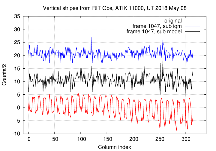
Image 1400:
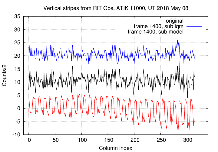
Image 1800:
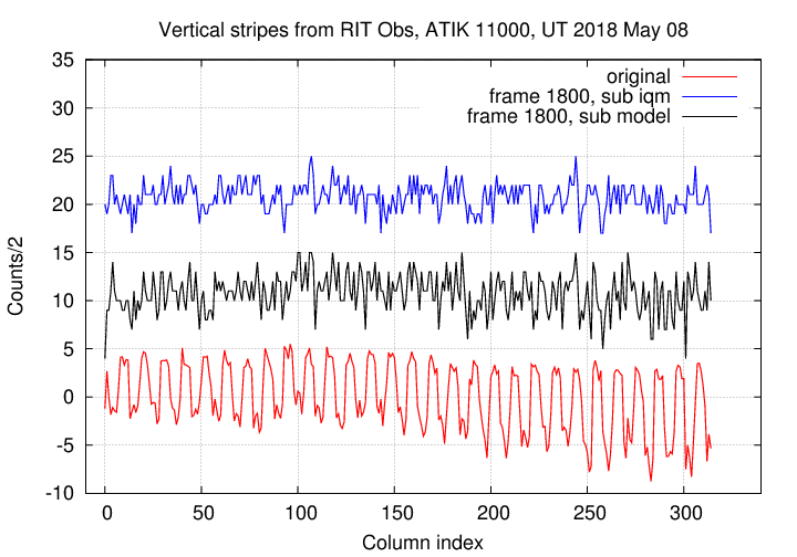
Again, the two methods are improvements over the original, un-corrected images. That's good. It appears to me that the blue lines in these images show slightly less residual variation than the black lines; in other words, using the master column vector seems to do a slightly better job than using an analytic model.
That small difference is borne out if we compute the mean and standard deviation from the mean for these post-subtraction column vectors.
           Standard deviation from mean of column vector (counts/2)

                    original       subtract master       subtract model
-------------------------------------------------------------------------
  frame 1047         3.70               1.54                  2.04

  frame 1400         3.63               1.60                  2.14

  frame 1800         3.72               1.47                  2.06
-------------------------------------------------------------------------
It does indeed seem that simply creating a master column vector from a large set of images, and then subtracting it from each image, is the best way to remove the "vertical stripe" artifacts.
Last modified 5/21/2018 by MWR.