On the night of June 3/4, 2013, I observed the active galactic nucleus (AGN) NGC 6418 (for an ongoing research project on reverberation mapping) and the brand-new cataclysmic variable star PNV 19150199+0719471. I spent most of my time on the second object, which is in outburst now.
The setup was:
Notes from the night
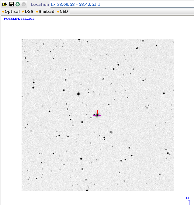
First target, the AGN NGC 6418.
Target 1: NGC 6418. RA = 17:38:09.53 Dec = +58:42:51.
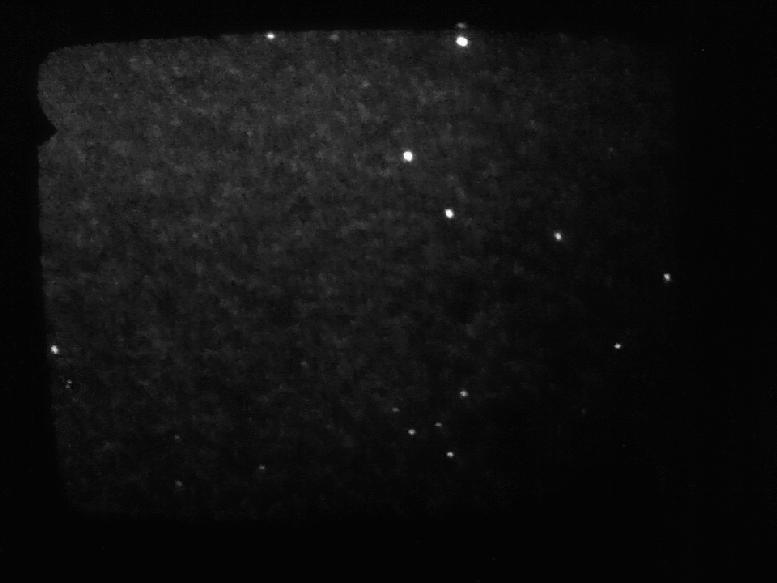
When I was on NGC 6418, the the guider telescope field looked like this:
I took a series of twenty 120-second guided exposures, and discarded 3 which were slightly trailed. Below is a stacked median image, 17 x 120 seconds in V-band. The field of view is about 15 arcminutes across, with North up, East to the left. NGC 6418 is the slightly fuzzy object just to the right of a medium-bright star at upper right.

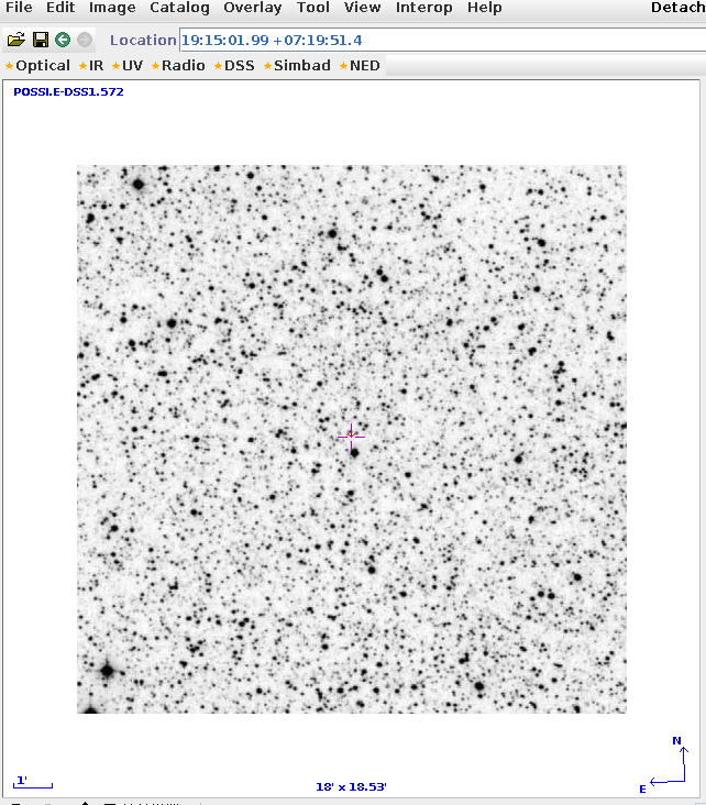
Target 2: the cataclysmic variable star known as PNV 19150199+0719471. Patrick Schmeer wrote an early message summarizing some of the information about it:
PNV J19150199+0719471

Newly discovered probable WZ Sge-type dwarf
nova in Aquila, currently at magnitude V=10.6
(discoverer: Koichi Itagaki (Yamagata, Japan)).
http://www.cbat.eps.harvard.edu/unconf/followups/J06270375+3952504.html

Astrometry and photometry by Enrique de Miguel:
R.A. 19:15:02.047 decl. +07:19:46.78 (J 2000.0)
2013 June 1.01 UT, V = 10.56, B = 10.40 (private message).

The blue colour and the large proper motion indicate that
PNV J19150199+0719471 (= IPHAS J191502.09+071947.6?)
is probably a dwarf nova in outburst (Taichi Kato,
vsnet-alert 15768).

According to the PPMXL catalog this object has a
large proper motion:
pmRA = -97.4 mas/yr and pmDE = -93.8 mas/yr.

PNV J19150199+0719471 is probably not a nova but
a nearby WZ Sge-type dwarf nova in outburst.
Spectroscopy and time-resolved photometry are strongly
recommended.
Here's a chart from the Digitized Sky Survey.
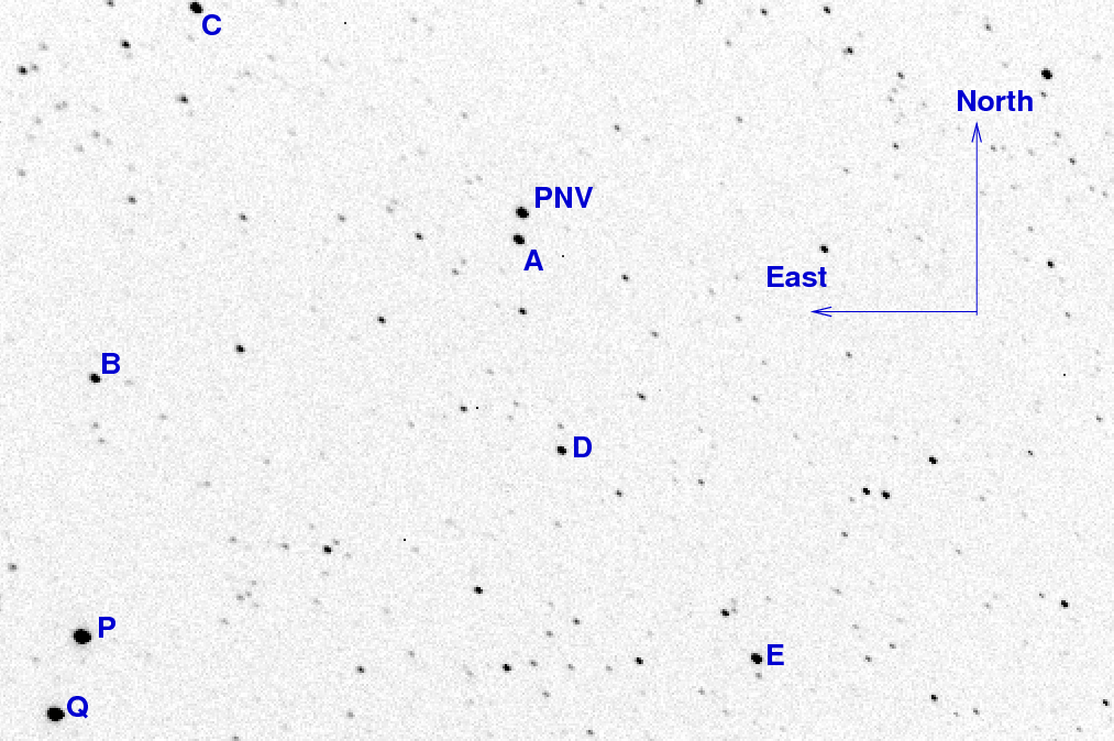
Last night, when pointing at the field, the guider telescope field looked like this:
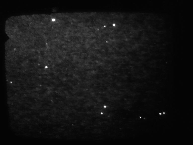
Putting the target object near the middle-top of the field, so that the two bright stars P and Q (HD 180219 and BD+06 4070) just peek into the southeastern corner of the field, yields a pretty good guide star. I took a set of 20-second guided exposures. Quite a few suffered from some trailing, especially as the object approached the meridian. I discarded many images, leaving 346 good images out of an original set of 432. I'll try using a different guider cadence (last night used a 4-sec exposure, I think) next time.
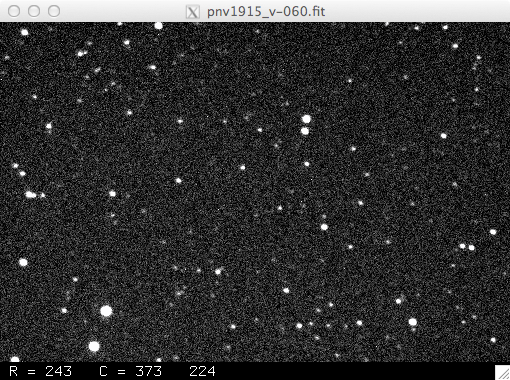
Below is one of my images.
Using aperture photometry with a radius of 4 pixels (radius of 7.4 arcsec), I measured the instrumental magnitudes of a number of reference stars and the target. Following the procedures outlined by Kent Honeycutt's article on inhomogeneous ensemble photometry, I used all stars available in each image to define a reference frame, and measured each star against this frame. I used the UCAC4 V-band magnitude for star "E" to convert the ensemble instrumental magnitudes to the standard V-band scale.
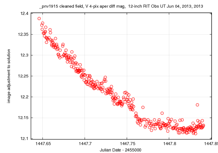
The graph below shows the change in zeropoint from image to image. The steady decrease is the sign of a clear night; the field rose in the east and reached a maximum altitude just as I quit due to dawn.
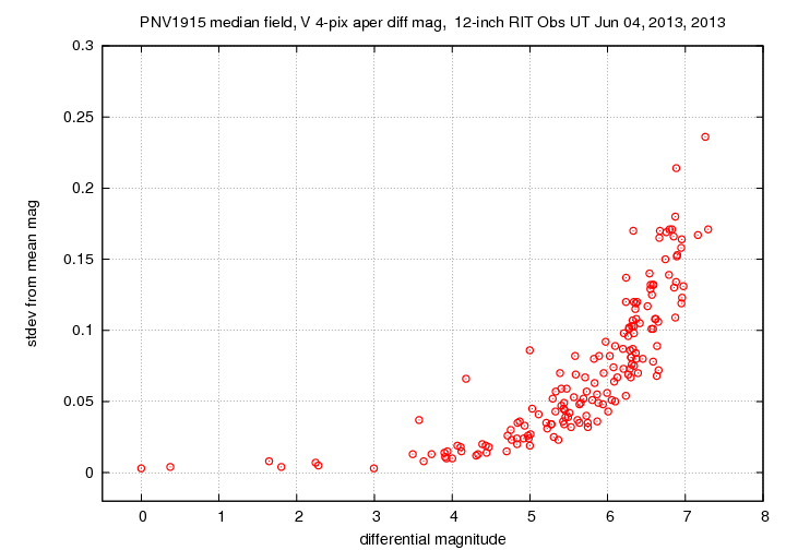
The scatter as a function of instrumental magnitude shows that the brightest stars had a scatter of roughly 0.005 mag; those two stars were slightly saturated. The target, at instrumental magnitude 1.8, has a slightly elevated scatter, compared to a star at instrumental magnitude 1.9.

The star with high scatter at instrumental magnitude 3.3 is a different real variable star. It is marked "B" on the chart above, and was listed as a variable by Bernhard and Lloyd, IBVS 4920, 1 (2000) . It is also known as GSC 00476-00295; it appears in dark blue in the graph below.
Here are light curves of the target star (green crosses) and some of the other stars in the field.
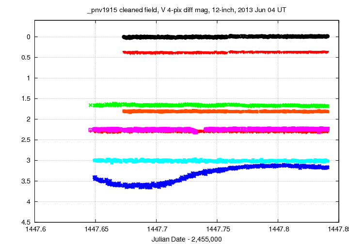
Here's a closeup of the target (green crosses) and a shifted version of star A (red symbols).

There _are_ some variations in PNV 1915, but their amplitude is only about +/- 0.02 mag, so they are just about swamped by the noise.
I sent a message to cba-data with the following report. This shows only the first few lines of measurements -- the full set can be retrieved using the link below.
# Measurements of PNV19150199+0719471 made at RIT Obs, Jun 4, 2010 UT,
#    in good conditions,
#    by Michael Richmond, using 12-inch Meade and SBIG ST-8E CCD.
# Exposures 20 seconds long, V filter.
# Tabulated times are midexposure (FITS header time - half exposure length)
#    and accurate only to +/- 1 second (??).
# 'mag' is a differential magnitude based on ensemble photometry
#    using a circular aperture of radius 7.4 arcseconds.
#    which has been shifted so UCAC4 487-093884 has mag=11.486
#    which is its V-band magnitude according to UCAC4.
#
# UT_day             JD            HJD        mag    uncert
Jun04.14591     2456447.64591  2456447.64993  11.332  0.009
Jun04.14910     2456447.64910  2456447.65313  11.339  0.010
Jun04.14955     2456447.64955  2456447.65358  11.343  0.009
Let me use some of tonight's images of PNV 1915 as a test for two methods of co-adding images. Since the conditions were good tonight, combining individual images in a simple way should yield decent results.
I'll begin with one image of the field: a single 20-second V-band exposure. None of the stars in this image are saturated, or even close to saturated.
How precise are measurements made with exposures like this? We can check empirically by comparing the measurements of stars in 10 consecutive images. Noiseless data would yield exactly the same value for each star, but real measurements will show some scatter. The brighter stars ought to have smaller scatter, since their signal-to-noise ratio is higher.

This shows the expected pattern. The brightest stars in the field have a scatter of about 0.008 mag.
Now, let's talk about combining images. Before I did any combining, I shifted individual images by small amounts in order to align the stars.
One way to combine images is to add them. Below is the straight sum of 10 consecutive images from the middle of this run. I've tried to set the contrast so that the background noise has roughly the same appearance as in the original image.
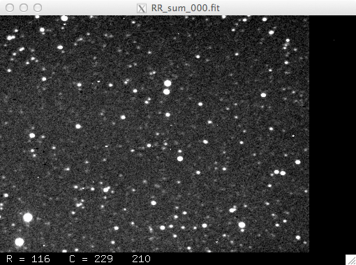
There are clearly more stars visible in this image. The black area at the right edge marks a position which wasn't covered by all 10 images, due to a small shift in the pointing.
I created 10 summed images, each composed of 10 original images -- in other words, I analyzed a set of 100 original images. We expect that, with higher signal-to-noise, the scatter between measurements of a star in these summed images should be smaller than it was in the original images. And that's what we see. The brightest stars now have a scatter of only about 0.003 mag.

Another way we can combine images is by taking the median value at each pixel location. This method should be less affected by big outliers than the simple sum.
Below is the median of 10 consecutive images from the middle of this run (the same set of 10 as I used to create the summed image above). I've tried to set the contrast so that the background noise has roughly the same appearance as in the original image.
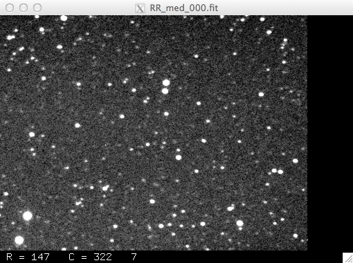
There are more stars visible in this image than in the original. In addition, this image shows fewer "hot pixels" -- high single pixel events -- than the summed version. The black area at the right edge again marks a position which wasn't covered by all 10 images, due to a small shift in the pointing.
I created 10 median images, each composed of 10 original images -- in other words, I analyzed a set of 100 original images. Let's see how precise the measurements of these images are when we analyze the entire set. The brightest stars in this analysis have a scatter of about 0.004 mag -- just a little bit higher than the summed version.
It will be easy to compare the results if I simplify things a bit. I'll break the stars into bins of width 0.5 magnitude, and compute the median value of the scatter of all the stars within each bin.
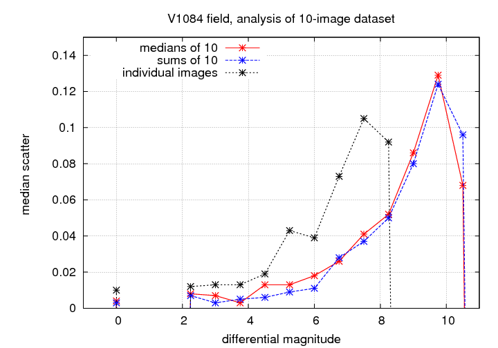
So the combined images do show a smaller scatter at a given magnitude than the original images. In theory, the scatter ought to decrease by a factor of the square root of the number of combined images; here, that was 10, so we might expect a decrease in the scatter by a factor of 3.2 or so. The actual decrease is a bit smaller -- more like a factor of 2 or 2.5 -- but we're in the ballpark.
In this case, using a sum provides slightly better results. When the original data is noisier -- for example, if it includes satellite trails, or strong cosmic ray hits -- the median method may yield better results overall.
Last modified 05/26/2013 by MWR.