The TESS and AAVSO are putting together a team of ground-based observers who can perform followup studies of exoplanet candidates found by TESS. People who want to join the team are asked to analyze a "practice" dataset, which can be found at the astrodennis.com website. I decided to give their second test a try.
The procedures followed herein are described more fully in my account of analyzing the first test dataset.
Contents:
The first step is to create "master" calibration frames. The dataset contains
All raw images are 16-bit integer FITS files, with 1375 x 1100 pixels. The camera was cooled to -30 C for all images.
I used the XVista image processing package to do the work. One of its limitations is that it can only handle 16-bit integer data, in the range -32768 to +32767 counts. In order to prevent some bright stars with pixels between 32768 and 65535 from overflowing, my first step was to divide all raw images (calibration and science) by 2. Therefore, all pixel values quoted below in darks and flats will have values which are half the value one would derive with other software. Since there are plenty of bits of noise due to the sky background, this won't affect the science results to any significant degree.
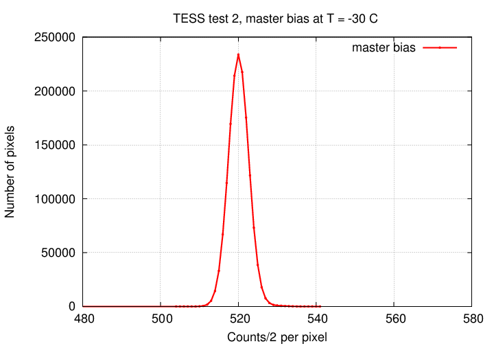
The next step was to combine all the bias images into a master bias frame. We'll need that frame, plus the master dark frame, to remove the dark current from flatfield images. Using an interquartile mean algorithm, I created a master bias image. The histogram of pixel values looks like this:
Next, we need to create a "master dark" frame. Now, what we really need are two master dark images: one for the science frames (20 seconds long), and another for the flatfield frames (3 seconds long). The second must be an image which will allow us to compute the contribution of the dark current to an image of any exposure time. What we have are a set of 20-second darks. So, the plan is
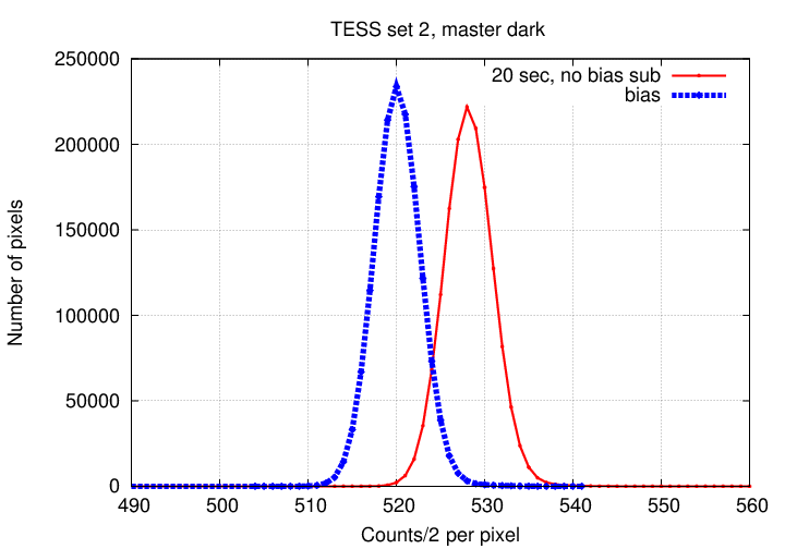
The combined 20-second dark image (= "master_dark_20") has a histogram of pixel values which has a peak at a SLIGHTLY larger value than the master bias:
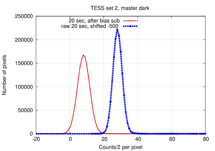
Subtracting the master bias from the combined 20-second dark image yields our "master_current_20" frame. Its histogram of pixel values has a peak of just a few counts, because this chip doesn't generate very much dark current per second. The figure below compares the histogram of this "master_current_20" to the histogram of the original combination of the 20-second images alone. Note the slightly broader peak in the "master_current_20", due to the random noise in the master bias frame which we subtracted from it.
Finally, we come to the flatfield frames. Since these have an exposure time of 3 seconds, in order to subtract the dark current properly we need to do a bit of algebra. For each pixel in every raw flatfield image, we compute
                               (                                        3    )
 cleaned_flat  =  raw_flat  -  ( master_bias  +  [ master_current_20 * --- ] )
                               (                                       20    )
Then, having cleaned our flats, we combine with an interquartile mean to create the "master flatfield" image. It turns out to have a mean value of 16014 counts, and looks like this: North is up, East to left. The greyscale runs from black = 14000 counts (and lower) to white = 17000 counts (and higher).
![]()
The master flat shows several features of note:
This is pretty simple. All the science frames are 20 seconds long, so we can get rid of the dark current by subtracting the "master_dark_20" image. Then, we can perform the flatfield correction by dividing by a normalized value of the "master_flat" image. In other words, on a pixel-by-pixel basis
               ( raw - master_dark_20 )
 cleaned =     -------------------------- * (mean_of_master_flat)
                    ( master_flat )
Even the raw images look pretty nice to the eye, but the clean images look even nicer. Aside from a few hot pixels which aren't completely removed by the dark subtraction, the images are quite pretty:
![]()
Let's add a few labels to provide orientation and identify some stars for later reference.
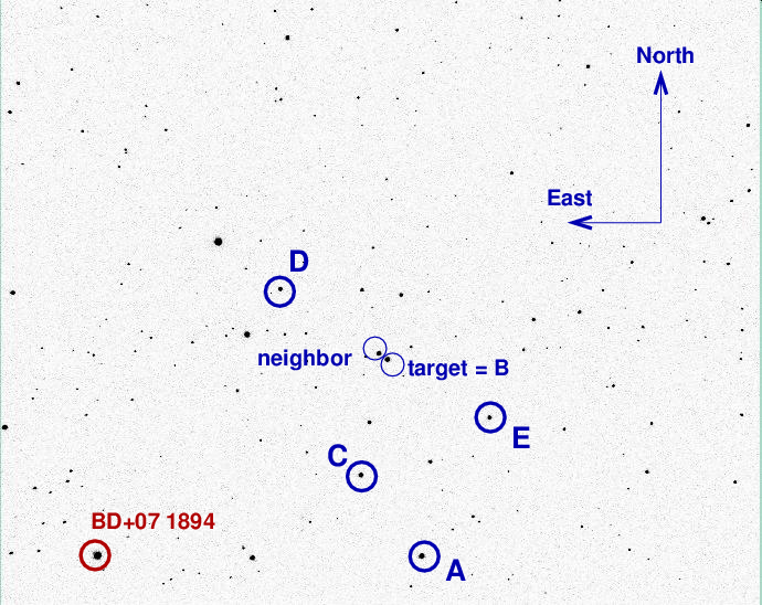
This is a good point to mention one complication: the telescope used to acquire these images was evidently a German equatorial design, because it paused briefly to flip itself over at the meridian. Images 1-285 had one orientation, and and image 294-484 were rotated by 180 degrees relative to the first set. I un-rotated the latter images so that all images had the same orientation before proceeding.
We can measure the brightness of stars in these clean images using aperture photometry. How big should we make the aperture? I checked the FWHM of stars in a few images, and found
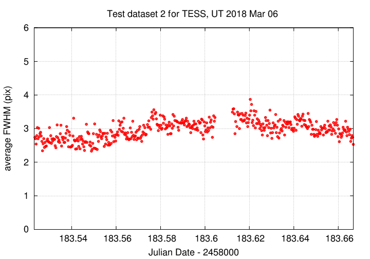
The change in size of the PSF across the frame would make absolute photometry difficult, but since we only care about changes in the brightness of each star throughout a set of continguous images on one night, it doesn't matter to us. I chose three apertures, of radius 4, 6, 8 pixels. In all cases, I used a annulus of radii 15 and 30 pixels to determine a local sky background.
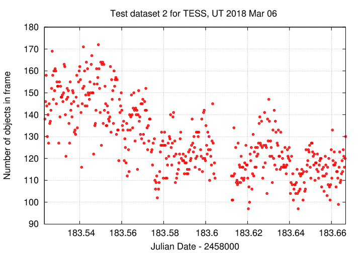
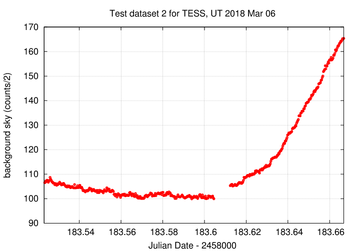
I then measured the brightness of every star with a peak at least 15-sigma above the background in every frame. This typically yielded 100 to 150 stars. The number decreased later in the run due to a higher background sky value.
The science images consist of a set of around 470 images, taken as the field gradually moved across the sky, starting at airmass 1.286, crossing the meridian, and ending at airmass 1.281. I'm guessing that the western sky has more buildings and lights than the eastern sky; the latitude and longitude in the FITS header support this guess, as they indicate the telescope is located in Annapolis, MD, just east of Washington, DC.
So, we now have measurements of the instrumental magnitude of some 100 to 150 stars per image, for some 470 or so images. What do we do with all this information?
I prefer to employ inhomogeneous ensemble photometry, which uses every star available in every image to create a photometric reference system. Each star is then compared to this overall photometric reference system, yielding differential magnitudes for all stars at once. You can read more about the procedure in Kent Honeycutt's article on inhomogeneous ensemble photometry, and at the home page for the software I wrote to implement it.
One of the outputs of the ensemble photometry procedure is a measure of the magnitude zero-point offset of each image, relative to some arbitrary reference; in other words, how much did the magnitudes of ALL the stars in one image appear to shift brighter or fainter, compared to the magnitudes of all the stars in other images? A graph of this quantity over the course of the run can reveal the presence of clouds or other photometric variations. In our case, we see a general trend for which falls and rises as the field rises, then falls, past the meridian; this is due to the changing airmass and extinction. I see no evidence for clouds.
![]()
A second quantity generated by the ensemble photometry procedure is a measurement of the scatter around the mean magnitude of each star. If we plot this scatter against the mean (differential) magnitude of each star, we expect to see small values for bright stars, and large values for faint ones. The results for this dataset look as we expect, with a few exceptions.
![]()
The floor of this distribution is about 0.006 mag, but there are two outliers:
Having made those changes, I re-ran the ensemble procedure to generate a fresh photometric solution. I then made a graph showing the light curve of the target (B), its neighbor, as well as light curves of a few relatively bright stars. We can use these light curves as a check to make sure we haven't left some systematic errors in the results.
In the graph below, I've performed a very rough photometric calibration using star "A" = TYC-206-524-1 to convert the differential, unfiltered magnitudes onto the V-band magnitude scale.
![]()
What do we see?
Now, if the light from both the target, and the neighbor, were to fall into a single big aperture, then the combined light would
If we add up the light from those two stars, based on our measurements, and convert them to a magnitude, we get the light curve shown in small black symbols ("combined") below.
![]()
Note that the depth of this variation, about 0.05 mag, is considerably larger than the prediction of 16.4 mmag = 0.0164 mag. Perhaps the aperture in TESS's measurements only incorporated a fraction of the light of the neighbor ...
The separation of the two stars is about 19 arcsec. Since the TESS pixels are about 21 arcsec in size, the light of these two stars will end up being mixed together in some way.