 Copyright © Michael Richmond.
This work is licensed under a Creative Commons License.
Copyright © Michael Richmond.
This work is licensed under a Creative Commons License.
Table of contents:
Tony George observed the asteroid (11072) Hiraoka occult the star TYC 0789-00349-1 on UT May 23, 2006. He watched from his driveway in Umatilla, Oregon, near latitude +45.9336, longitude 119.2986 West. His equipment included
  Meade LX200GPS 12-inch Schmidt-Cassegrain telescope
  Meade f3.3 focal reducer
  PC164C CCD video camera
  STVAstro GPS video time inserter
  Garmin 16 GPS
  Canon ZR50 Mini DV tape recorder
Tony has analyzed the videotape using LiMovie, going field-by-field (each field is 1/60 of a second). He found evidence for a brief occultation, lasting only 14 fields.
He asked me to examine the video, just to confirm his measurement.Below is a picture which represents 100 coadded images. I have added labels for three stars:
  star   Tycho-2 ID     RA            Dec           Vt
-------------------------------------------------------
   A   0793-00003-1   08:06:09.173  +13:08:50.75   9.7

   B   0793-00349-1   08:06:06.589  +13:11:36.64  10.5

   C   0789-00349-1   08:06:01.653  +13:05:40.94  10.7   Target
-------------------------------------------------------
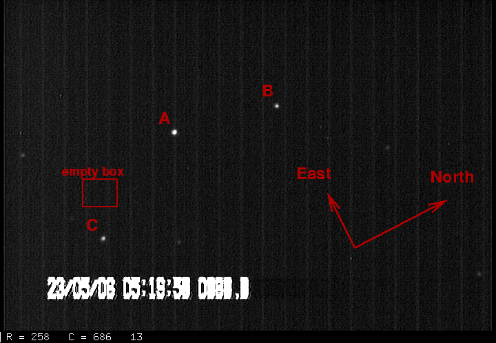
I also show an empty box, placed just above the target star "C". I'll use that empty box as a measure of blank sky.
Here's a view of one of the video frames rotated so that it is in the standard orientation.

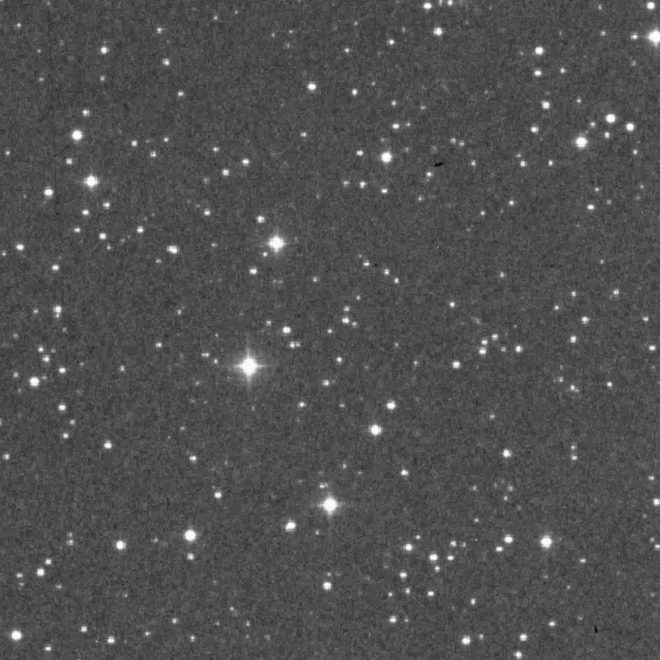
Compare it to a section of the Digitized Sky Survey below, which is 15 arcminutes on a side:
Tony's full video recording covers about 6 minutes; he broke this very long record into 6 movie files, each covering about one minute. I analyzed only the minute surrounding the event, which corresponds to his file "B". The first frame in this clip corresponds roughly to UT 05:19:52.86. Tony can provide much better information on the times since he has analyzed the video stream field-by-field.
First, I broke the video clip into individual frames, using TMPGEnc The result was a set of JPEG images, each 720 x 480 pixels in size. Each frame had a KIWI OSD timestamp at the bottom. My analysis used frames, composed of two superimposed fields, so the timestamp was a blurred version of the stamps on two consecutive fields.
In order to process the data, I
There were several stars visible in the video. I chose the brightest, which I call "A" in the charts above, as a primary reference. Star "B" serves as a check on star "A". The empty region shows what sort of "signal" will appear from a blank piece of sky; if all goes well, it will produce zero integrated light.
For each of the frames, I
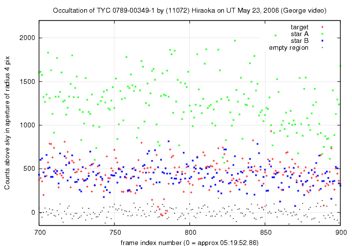
Here are quick views of the results. I decided that the aperture with radius 4 pixels gave the best results, so I show them in the plots below. You can find measurements through two other apertures in the table at the end of this section.
First, the entire light curve for the three real stars:

Note that the target star does appear to fade to zero light briefly, just before frame 800.
Now, let's look at region around this event. I'll include measurements made of the "empty box" to the side of the target star.
We can zoom in even closer:
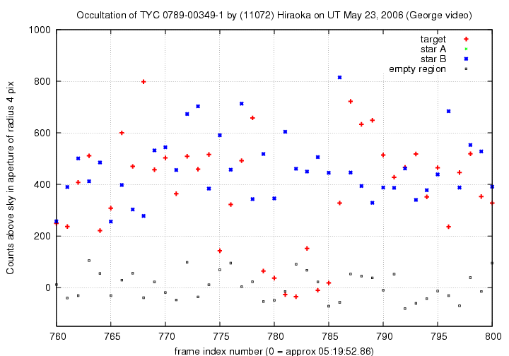
My photometry shows 7 consecutive frames in which the signal from the star is far below its usual level; in 6 of these 7 frames, the signal is consistent with the light in the "empty box". The seventh measurement is _just_ above the largest "empty box" measurement.
I agree with Tony's conclusion: the asteroid occulted the star for 7 frames, which is equivalent to 14 fields.
You can grab the data in multi-column ASCII text files below. The columns are
 col              quantity
------------------------------
  1              frame index

  2,3            flux of reference star "A" in 4-pixel-radius aperture,
                     and estimate of uncertainty in that flux
  4,5            ditto 5-pixel aperture
  6,7            ditto 6-pixel aperture

  8,9            flux of check star "B" in 4-pixel-radius aperture,
                     and estimate of uncertainty in that flux
 10,11           ditto 5-pixel aperture
 12,13           ditto 6-pixel aperture

 14,15           flux of target star in 4-pixel-radius aperture,
                     and estimate of uncertainty in that flux
 16,17           ditto 5-pixel aperture
 18,19           ditto 6-pixel aperture

 20,21           flux of empty region in 4-pixel-radius aperture,
                     and estimate of uncertainty in that flux
 22,23           ditto 5-pixel aperture
 24,25           ditto 6-pixel aperture
An exchange of E-mails prompted me to do a little bit of statistical analysis. Since the dip in stellar brightness lasted only a small number (seven) of frames, how confident can we be that it was really due to an occultation, rather than by some sort of random noise in the signal?
I have gone back to my analysis of this occultation to see if there is any way to quantify the probability that the putative event indicated between frames 778 and 785 in my indexing scheme might be real, or just an artifact of random noise.
First, I looked at the check star I labelled "B", which has roughly the same brightness as the target star. The statistics of my photometry within a circular aperture of 4 pixels (after subtracting a local sky background) are
N = 1799 frames mean = 431 RMS = 127
If these measurements are drawn from a random gaussian distribution with mean 431 and standard deviation 127, then we would expect a particular fraction of the values to lie within certain ranges. In particular
       -1 to +1 stdev       expect                 actual
 --------------------------------------------------------------
      305 to 558           68 % = 1223 frames      1244 frames

      177 to 685           95 % = 1717             1714

       50 to 812         99.7 % = 1794             1796
---------------------------------------------------------------
The measurements of star C appear reasonably consistent with a random gaussian distribution, although there are more values near the peak of the actual distribution than the true gaussian. The wings of the distributions appear very similar.
Now, let's look at the target star. I will exclude the frames around the time of the putative event, compute some statistics, and again compare to a random gaussian distribution.
N = 1758 frames mean = 478 RMS = 143
If these measurements are drawn from a random gaussian distribution with mean 478 and standard deviation 143, then we would expect a particular fraction of the values to lie within certain ranges. In particular
       -1 to +1 stdev       expect                 actual
 --------------------------------------------------------------
      335 to 621           68 % = 1195 frames      1197 frames

      192 to 764           95 % = 1670             1681

       49 to 907         99.7 % = 1753             1751
---------------------------------------------------------------
I would again claim that the measurements are reasonably consistent with a gaussian distribution, of mean 478 and standard deviation 143.
Let us assume that the counts from the target star are indeed drawn from such a gaussian distribution. What are the chances that we might draw 7 consecutive low values? The highest of the 7 values during the putative event is 152 counts, so we'll use that as a marker.
     Q1:  What is the probability of drawing a single
          value less than 152 from a gaussian distribution with
          mean 478 and standard deviation 143?

          Answer:  normal deviate z = (152 - 478)/143  =  -2.28

                   Prob (1 value with z < -2.28)  =   0.0113


     Q2:  What is the probability of drawing seven consecutive
          values less than 152 from a gaussian distribution with
          mean 478 and standard deviation 143?

          Answer:  Prob (7 consecutive values with z < -2.28)

                     =  Prob (1 value with z < -2.28)^7

                     =  (0.0113)^7  =  2 x 10^(-14)
That's a very small probability.
Now, in any real set of measurements, there are more gigantic outliers than from a real mathematical gaussian distribution, due to voltage spikes, dust particles, wind shake, and all sorts of experimental errors. I would not take this cumulative probability too seriously, but it does indicate that the chances are very very low that _random_ noise would cause 7 consecutive low values. Some unknown _systematic_ effect could very well do so, of course. But would it occur at very close to the predicted time of occultation? Let us continue. Suppose that we suspect the putative occultation really did take place. In that case, the counts within the aperture should represent empty sky only. If you examine my report on this event, you'll see that the coadded frames of the video show a series of lightish vertical stripes throughout the frame. One of those bands lies just to the side of the target, about 8 pixels to the right. This band is outside the aperture used to measure light of the target, but inside the annulus (inner radius 10 pixels, outer radius 20 pixels) used to estimate the background sky value. The combination of this lightish stripe and the darker regions of sky surrounding it could give rise to an unpredictable background signal ...
I measured the light in a region of the sky not far from the target star, called the "empty box" in my report. Let's look at the statistics of counts in that portion of the sky, since they might be similar to counts from the sky under the target.
N = 1799 frames mean = -2 RMS = 59
If these measurements are drawn from a random gaussian distribution with mean -2 and standard deviation 59, then we would expect a particular fraction of the values to lie within certain ranges. In particular
       -1 to +1 stdev       expect                 actual
 --------------------------------------------------------------
      -61 to  57           68 % = 1223 frames      1250 frames

     -120 to 116           95 % = 1717             1722

     -179 to 175         99.7 % = 1794             1796
---------------------------------------------------------------
Again, there are more values close to the center of the distribution than in a true gaussian distribution, but the wings are similar.
The highest count rate during the putative event is 152 counts.
     Q1:  What is the probability of drawing a single
          value of at least 152 from a gaussian distribution with
          mean -2 and standard deviation 59?

          Answer:  normal deviate z = (152 - (-2))/59  =  +2.61

                   Prob (1 value with z > +2.61)  =   0.0045


     Q2:  What is the probability of drawing at least one value
          of 152 or more in a set of seven consecutive trials
          from a gaussian distribution of mean -2 and standard
          deviation 59?

          Answer:  Prob (at least 1 of 7 having z > +2.61)

                     =  1  -  Prob (7 values with z < +2.61)

                     =  1  - [ (0.9955)^7 ]

                     =  0.031
That's a small probability -- one chance in 32. But it is much, much higher than the probability derived earlier that random noise in the light from the target star would lead to 7 consecutive values as low as those observed.
I conclude that a statistical view favors the interpretation of an occultation. Again, let me remind us all that the statistics apply only to random fluctuations. Systematic errors (a bird flies through the telescope beam, etc.) will invalidate all these statistical results.
Finally, I went back to the individual video frames and examined the ones during the time of putative occultation carefully, to see if I could notice any hot pixels, or image defects of any kind. After spending 15 minutes looking at sequences of images at several different contrast levels, I decided that I can clearly see the target star in frames up to 778, and after 787. In frame 786, the star is present, but looks less distinct to my eye. In the intervening frames 779 to 785, I see no evidence for starlight. I examined very carefully frame 783, the one giving rise to the single high point during the putative occultation; I can't see any obvious image defect. The compression algorithm used by the video camera or recording device does leave the entire frame littered with little blocky features, all the time, and that made it hard to see anything out of the ordinary unless it was _really_ out of the ordinary.
My conclusion: occultation is the most reasonable explanation of the video record.
Copyright © Michael Richmond.
This work is licensed under a Creative Commons License.