 Copyright © Michael Richmond.
This work is licensed under a Creative Commons License.
Copyright © Michael Richmond.
This work is licensed under a Creative Commons License.
What happens when the limb of the Moon passes in front of a distant star? What should we expect to see? Obviously, the star changes from bright (before the limb comes close) to invisible (after it is completely hidden by the limb), but if we could measure its intensity very carefully, what details might we expect to see?
I will attempt to give a very basic introduction to the topic in this document, together with some simple examples which may serve to provide a flavor of the sort of phenomena one might expect in real life. Those who are interested in the details should probably consult a university textbook on optics. I will mention several complicating factors, but treat none in great detail.
I'd like to thank Roger Easton, of RIT's Center for Imaging Sciences, for his advice and guidance on this problem. Thanks also to Brian Loader for catching an error in the horizontal scale of graphs in the section on partially resolved disks.
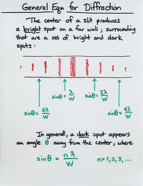
You may be familiar with the phenomenon of diffraction: the interference of waves from a source when they encounter an obstruction. We use the example of light passing through a slit and falling on a distant screen to illustrate the effect in our introductory physics classes:
In the case of monochromatic light passing through a narrow slit onto a distant screen, we find a simple pattern of light -- fringes of constant spacing -- on the distant screen. There's even a simple formula relating the wavelength of the light and the width of the slit to the angular size of the fringes. How convenient ....
When the Moon passes in front of a star, it also produces diffraction. But the situation is a bit different: this time, light passes through a "slit" which has only a single edge:
The result, it turns out, will again be a set of fringes falling onto the distant surface of the Earth:
But this time, the fringes will not have a constant spacing, and the mathematical formula required to calculate their location and amplitude will not be so easy; moreover, as the Moon's limb moves through space, the pattern of fringes will glide across the ground.
The term "Fresnel diffraction" is often used to describe situations like the lunar occultation: a distant source of light sends waves past an obstruction of some kind and onto a distant screen. Now, there are several natural lengths in this problem:
How do these lengths combine to interact? It turns out that the crucial combination is the square root of the product of L and λ,
which I will denote by the lower-case letter b. This gives the characteristic spacing between fringes on the Earth's surface, and so can be compared with x, the distance on the surface away from the geometric shadow's edge.
For our particular case of a lunar occultation observed in the visible, b is typically
       b  =  sqrt [ L * λ ]

          =  sqrt [ 384 x 10^(6) m  *  500 x 10^(-9) m ]

          =  14 m
If we look at very large regions of the Earth, on scales x >> b, then the situation is simple: far from the geometric shadow's edge, for positive x the Earth's surface is uniformly bright; far within the geometric shadow, for negative x, the Earth's surface is completely dark. But in between, near the geometric shadow's edge on scales of meters or tens of meters, the brightness of the Earth's surface will vary in a complicated manner.
The goal, then, is to calculate the intensity of light falling on the Earth's surface at a distance x from the shadow's edge. It turns out that we can do so using the following equation:
Here I0 is some normalization factor which scales the entire pattern. I will fiddle with it throughout the examples herein to yield roughly the same overall intensity for all situations, since it is the relative variations in the signal with position that concern us.
We can split this complex integral into two real integrals if we wish:
Note that one must add up the pieces of each integral BEFORE squaring the result.
In the examples which follow, I performed numerical integration on a grid of stepsize 0.1 meter, considerably smaller than the characteristic length scale of 14 meters. I then tabulated the values of I(x) every 0.2 meters.
So, what sort of pattern do we get? The simplest case involves light of a single wavelength -- I'll choose λ = 500 nm. If we were to float in a balloon high above our telescopes, we would see a pattern of light and dark fringes on the ground like this:

It is easier to see the quantitative behavior on a slice through the pattern:
Note that the intensity reaches a value of exactly one-quarter of its nominal value at the location of the geometric shadow's edge.
If we zoom in on the first few fringes, we can see that the distance between each fringe decreases as we move away from the shadow's edge.
We have so far considered the light from a star to be monochromatic: all of a single wavelength. However, real starlight is a mix of different wavelengths. How will that affect the observations of an occultation?
In order to illustrate the effects of polychromatic light on diffraction patterns, I will consider four cases:
In each of the polychromatic cases, I will approximate a true continuum of light by adding together contributions from 11 wavelengths uniformly spanning the passband. So, for example, the "narrow" case will be simulated as the sum of light of 500, 505, 510, 515, ..., 545, 550 nm. I give each contribution equal weight. In real life, stellar spectra would vary significantly over the entire visible range, giving some wavelengths more weight than others. My simulations here therefore provide a sort of "worst case" set of examples. I suspect that a typical CCD-based video camera, observing a typical star through a typical atmosphere, yields a passband which lies somewhere between my "intermediate" and "wide" examples.
So, what happens when we include light of more than a single wavelength? In a sense, we must add together the diffraction patterns of each wavelength; I will perform the addition within the complex integral (though the results of adding the results afterwards look very similar). Each wavelength of light will have its own characteristic linear fringe size on the ground.
Thus, the diffraction fringes created by each wavelength will be slightly different in size. When we add the patterns together, it is reasonable to expect some cancellation of the diffraction fringes; that cancellation ought to become more more significant as the passband grows wider.
Let's find out if that is true. Below is the fringe intensity for the monochromatic case:
Next, look at the pattern for the "narrow" case:
The "intermediate" passband:
Finally, the "wide" passband:
Here are all four models shown at once for quick comparison:
Note that in all the cases, the first fringe is significantly brighter than the nominal intensity. As the passband grows, however, subsequent fringes very rapidly decline into uniformity.
Just for fun, we can look at the fringes as they would appear on the ground to an observer floating high above; from the very sharp, monochromatic case:
to the narrow band:

to the intermediate band:
 and finally the wide band:

Note added Mar 21, 2018: It appears that I made a small error in the calculations in this section. Although the text states that the star in this example is 10 milliarcsec in diameter, it seems that my calculations used a disk only 5 milliarcsec in diameter; probably a confusion of radius and diameter. Sigh. Thanks to Tarek H. for his detective work!
Although stars are so far away that they appear as point sources to the naked eye, some are close enough and large enough that their angular size produces detectable effects. Let us see what happens if the light source occulted by the Moon's limb is not a point source, but instead a very small disk.
I will consider here only the simplest model of a star:
In real life, the apparent angular size of a star certainly does change with wavelength (generally growing with wavelength); moreover, the limbs of stars usually appear fainter than the central portions of their disks (an effect called "limb-darkening"). It is not too difficult to add these complications to the mathematical computations described below.
There are (at least) two ways that we can modify our calculations to incorporate the non-zero angular size of a light source. They ought to (and do) produce the same results, but one method turns out to be a lot quicker in this simple case.
We then create a second, smaller image, which I'll refer to as "the 2-D kernel". This should be the projection of the angular distribution of the light source onto the Earth's surface.
A uniform disk of angular size θ will turn into a filled circle of linear diameter D on the Earth's surface, where
The 2-D kernel is simply a picture of this circle on the ground. For example, given the standard distance L = 384,000 km, a star of angular diameter θ = 1 milliarcsec produces a circle of linear diameter D = 1.86 m. The 2-D kernel for a star of angular diameter 10 mas ("mas" is the abbreviation for "milliarcseconds") would be a circle of uniform brightness with diameter 18.6 meters across. The figures below were probably made with a disk of angular diameter only 5 mas. MWR 3/21/2018

We then convolve the picture of the fringes with the picture of the 2-D kernel. In other words, we move the 2-D kernel all over the picture of the fringes, smoothing the picture with the kernel. We find afterwards a slightly fuzzier picture:

We can now look at the intensity in this convolved picture as a function of distance from the shadow's edge to figure out the new appearance of the fringes.
Once we have the 1-D kernel, we can apply it to the 1-D fringe pattern. This convolution is much quicker than the two-dimensional version.
In essence, we are smearing the 1-D fringe pattern over the width of the 1-D kernel.
In theory, the 1-D and 2-D convolution methods should yield the same result. Let's check to see if that's true. I'll pick a uniform circular disk of diameter 10 mas, which corresponds to about 19 meters on the ground, and look at the fringe pattern observed through a wide bandpass of 400 to 800 nm. The figures below were probably made with a disk of angular diameter only 5 mas. MWR 3/21/2018
Good. Both methods show the same result: the first positive fringe is still far above the normal intensity level, but subsequent fringes have been smoothed almost to invisibility. For convenience, I'll use 1-D convolution to create the following illustrations.
Let's now watch the fringe pattern change as the uniform disk grows larger and larger. Again, the setup is a wide optical passband and the Moon at its average distance.
Zooming in on the region near the first fringe shows more clearly the difference between disks of different sizes:
To do the best job of estimating the size of a star based on occultation data, one ought to compare full-blown models of the fringe pattern against the observations. But if one wants to make a quick estimate of the angular size of a disk based on the fringe pattern, one might use the height of the first fringe as an indicator. If we can measure accurately the intensity of the first fringe (see warning below) and the intensity of the star far from the shadow's edge, we can use the ratio of intensities to guess at the angular size:
Warning! Warning! In order to measure the intensity of the first fringe accurately, one must sample the light faster than it varies signficantly. That means on timescales of milliseconds, for a typical lunar occultation (see the section below for the conversion of distance to time). Remember that video rate is not fast enough to resolve the fringes in a head-on occultation; a video system would integrate the changing light across one or two fringes, which would drastically decrease the amplitude of the first fringe and lead to a large over-estimate of the angular size of the star.
Let us now turn to the specific case of lunar occultations, in which the limb of the Moon passes in front of a star. I will assume throughout this section a "typical" observing setup:
For the rough purposes of this discussion, I will continue to assume that an effective value for characteristic size of the fringes b is about b = 14 meters.
How fast will the Moon's limb move across the pattern? It depends on the angle at which the surface approaches the star. Let us denote the angle between the very leading edge of the Moon and the point on its limb which first touches the star by the letter a.
Then the lunar limb will move across the star with a velocity which is V cos(a).
The speed of the Moon through the sky varies with the position of the Moon in its orbit, but we can find an approximate value without too much difficulty: if the Moon makes one complete revolution through the sky every 27.3 days, then it must move with a linear speed
           2 * pi * 384,000 km
    V  =  --------------------    =   88,379       km/day
              (27.3 days)

                                  =    3,682       km/hour


                                  =        1.02    km/second


                                  =     1000       m/second   approx
For very rough purposes, the Moon's shadow and its entire fringe pattern will glide across the Earth's surface at about 1000 meters per second; that's not too hard to remember.
In order to simulate accurately the fringes observed during a particular event, one must do a better job of calculating the speed of the fringes across the landscape. This involves accounting for
One relatively simple way to incorporate these factors is to use a good planetarium program to measure the Moon's angular motion in the sky as seen from the observing location for, say, an hour before the occultation to an hour after the occultation. One can use the difference in position to calculate the apparent angular motion of the Moon relative to the star, and use that apparent angular motion times the Earth-Moon distance L at that time to calculate the linear speed V of the fringes across the observing site.
- the motion of the Moon in its orbit
- the rotation of the Earth
- the position of the observer on the face of the Earth relative to the sub-lunar point
Recall that for our "typical" setup, the characteristic angular size of the fringe pattern is about b = 14 meters. So, if a star lies directly in the Moon's path, and is covered by the very leading edge of the limb, the first fringes will zip past in very roughly (14 m)/(1000 m/s) = 0.014 seconds. This is less than the duration of a single video frame. We must conclude that ordinary video cameras will not resolve the fringes in a direct lunar occultation.
In order to calculate the measurements made by a video camera, one would have to integrate the intensity over the duration of a video frame; in other words, break up the fringe pattern into chunks of size N meters, where "N" corresponds to the speed of the fringe pattern times the duration of a video frame (i.e. 1/30 of a second). There would be some ambiguity in exactly where the bins should start, so one would have to run several models and see which fit the video record best.
On the other hand, if the Moon's limb slides past a star at a grazing angle, then the speed of the fringe pattern can decrease dramatically. If the star is first touched when at an angle a from the leading edge, then the ground speed of the fringe pattern is
V = 1000 cos(a) m/s approx
So, for example, if a = 87 degrees,
then the ground speed slows to
only about 52 m/s,
and the first few fringes will
each take roughly
0.27 seconds = 8 video frames
to pass.
So, we can now go back to some of the graphs
shown earlier in this document and figure
out the duration of specific features.
For example, look again at the signal from
a point source in a wide passband:
Warning! Warning! Danger, Will Robinson!
It may not be a simple matter to compare
actual video measurements
to these theoretical predictions
if the recording procedure introduces
a non-linear response.
For example,
if the uncovered star
saturates the video camera,
then the recorded brightness will not
appear to drop as soon as the real brightness
does begin to decrease.
Even if the camera does convert the starlight
into a video signal in the proper linear fashion,
that signal may not be recorded properly
on a videotape.
Finally, the procedure by which one
analyzes the recorded movie --
whether judging the brightness by eye,
or via the diameter of the star's image on a
monitor, or by digitizing each frame
and integrating the light through an aperture --
may introduce additional non-linear effects.
The bottom line is that there are several mechanisms
by which the true intensity of the star may
be distorted.
Most of these mechanisms act
to reduce the dynamic range of the measurements,
compressing the range between
maximum light and minimum light
and decreasing the time over which the
change takes place.
There is another issue which also acts to
decrease artificially the durations
of recorded events: background noise.
The graph above shows the integrated light
from a star decreasing to a value of exactly zero.
A real instrument may have a "noise floor"
caused by variations in the background value,
fluctuations in voltage, atmospheric distortion,
and so forth.
In that case, when the star's light drops
to the level of the noise floor, it effectively
disappears ... before the light REALLY
reaches a level of zero.
For example, imagine a case in which
we are monitoring a very faint star during
an occultation.
Suppose that we look at a truly
blank region of the sky
and measure a signal B.
Suppose further that the noise fluctuations
are of size +/- s,
meaning that these measurements of the
blank sky
range between B - s and B + s.
Now, when we look at the unocculted
star, suppose that it is so faint
that its integrated signal I
is just twice as large as the scatter in the
measurements: I = 2 s.
Our measurements of the light coming
from its area of the frame (including the background)
will have an average value B + 2 s ;
in other words, we barely detect it above the noise.
As the Moon's limb approaches, and then
begins to cover the diffraction pattern
of the star,
the star's light decreases.
As soon as it drops to half its original,
unocculted value, to I/2 = s,
the total light measurement at its position
will fall to B + s,
and we will be unable to distinguish it
from a random fluctuation in the background sky.
So, there are (at least) two factors which distort the
timing of
a drop in brightness during
an occultation:
Both factors act to make the measured
duration SHORTER than the theoretical duration.
Note that if two observers standing side-by-side
have equipment with significantly different
characteristics (saturation level, background noise, etc.),
they may derive rather different
durations for the very same event.
Another way to view the measurements is by
converting time into angular distance on the sky.
The Moon moves at roughly
0.5 arcseconds per second
through the sky.
For a direct, head-on occultation,
during each millisecond of time, the Moon's limb
moves by 0.5 milliarcseconds.
The record of intensity as a function of time
then becomes intensity as a function of angular size;
with our "typical" parameters,
Occasionally, light curves of lunar occultations
reveal STEPS in brightness,
like this one of 70 Tau observed by Fekel et al.:
Step-like features are clear signs that
the star being occulted is a binary.
One can use the delay between the two drops
in brightness to figure out the angular distance
between the components,
and the amplitude of the step to figure
out the relative brightness of the components.
Finally, let's look briefly at a factor
which can be most important in practice:
can one measure the signal from a star
adequately at video (or higher) rates
to see any of these diffraction features?
We can do a very rough estimate here.
We will assume for these rough purposes that
the star Vega has an apparent magnitude = 0.
Now, through this very wide passband,
Vega produces a flux of about 3.6 million photons
per second per square centimeter
above the Earth's
atmosphere. Given the "typical" values above,
we can calculate the number of photons which will
be detected:
We can then make up a table showing the number of
photons we can expect to detect per millisecond
for Vega-like stars over a range of magnitudes:
You may think that the number of photons is still
large, even for a star of magnitude 10,
but remember that the background will also be
producing photons.
If we were looking at a star isolated in
a featureless background on a clear night,
a typical sky brightness might
be (mag 19 per square arcsecond),
corresponding to about 13 detected photons
per second per square arcsecond of background.
For a typical small-telescope aperture radius
R = 3 arcsec,
the background underneath the star
has an area of about 28 square arcseconds,
meaning a sky contribution of about 370
photons per second, or 0.37 photons per millisecond;
negligible, compared to the signal from even a tenth
magnitude star.
Unfortunately,
the Moon tends to brighten the skies around it
considerably.
I do not have any real data
on the brightness of the unlit surface of
the Moon,
but I'd be willing to bet that
scattered light from the lit portion
of the lunar surface will
increase the background enough to drown out
the signal from a faint star.
Some nice examples of lunar occultations recorded in the literature:
See also
Figure 1 from
Photoelectric observations of lunar occultations
by Fekel et al., AJ 85, 490 (1980).
                                    photons
 detected photons  =   3.6 x 10^(6) ---------  *  (490 sq.cm) * (0.3)
                                    s * sq.cm

                   =   530 million detected photons/sec       approx

                   =   530,000     detected photons/millisec  approx
    mag            photons/millisec      photons/(video frame)
  --------------------------------------------------------------
     0               530,000               17,000,000

     2                84,000                2,800,000

     4                13,000                  440,000

     6                 2,100                   70,000

     8                   330                   11,000

    10                    53                    1,700
  ---------------------------------------------------------------
For more information
Copyright © Michael Richmond.
This work is licensed under a Creative Commons License.