
 Copyright © Michael Richmond.
This work is licensed under a Creative Commons License.
The headlines scream Mudtown Maulers are on fire! Although their record for the season is even at 65-65, the team has won nine games in a row. Does that mean that the Maulers are favorites to win tonight's game, too?
If you believe that a baseball team can become hot, in some predicative way, you might answer "yes." On the other hand, if you believe that it's all just random chance, you might answer "no." Is there evidence to support either viewpoint?
I have analyzed the records of teams in the American League during the period 1961 - 2006. The sample contains 594 team-seasons, most of which involve 162 games. In this report, I'll try to use that dataset to address the question of whether a team's recent past has any bearing on its immediate future.
If you can't wait, my conclusion is there may be a very weak positive correlation between pairs of consecutive games, and less probably a weaker correlation with a length of three games, but certainly no correlation on a timescale of more than three games.
First, a brief digression on the topic of "correlation." I am going to use the autocorrelation function to compare a team's record to a shifted version of itself. Let me provide the mathematical equation first, then explain it.
Let W(i) = 1 if the team wins game number i during the season, W(i) = -1 if the team loses game number i, and W(i) = 0 if it ties that game. Then the autocorrelation function C is defined by

The symbol Δ represents an offset in games. If we choose Δ = 1, for example, the value C(1) will tell us how much the result of today's game affects the result of tomorrow's game. On the other hand, choosing Δ = 5 and computing C(5) will tell us how much the result of one game affects the result of the fifth game from now.
A short example may make this more clear. Let's focus on the value of C(1), the correlation of game i with game i+1; in other words, the correlation of one game with the next. Suppose the Maulers have a four-game stretch in which their record is
W W W L
If we replace every win (W) with a "1", and every loss (L) with a "-1", we have
1 1 1 -1
In order to compute C(1), we add up three values:
The sum of these terms is:
        C(1)  =  (1*1)  +  (1*1)  +  (1*-1)

              =    1    +    1    +   -1

              =    1
The larger the value of the correlation function, the closer the connection between the games in question. It may help us to interpret it if we also look at the correlation function for some other choices of Δ. For example, choosing Δ = 0 means
        C(0)  =  (1*1)  +  (1*1)  +  (1*1)  +  (1*1)

              =    1    +    1    +    1    +    1

              =    4
So C(0) = 4 and C(1) = 1. And, obviously, there SHOULD be a very close connection indeed between the result of one game and the result of the very same game -- so the big number makes sense.
It turns out that we can interpret the correlation function for some choice of Δ in the following manner:
There are some additional details in my calculations of the correlation function which probably aren't interesting to anyone but a real mathematician (who would undoubtedly criticize them severely), so let's move back to baseball.
Before we look at the results of running real historical baseball records through the autocorrelation function, let's think of some of the possibilities. How could the results of one game affect those of the next? These are some silly examples, but I hope that they will provide some insight.
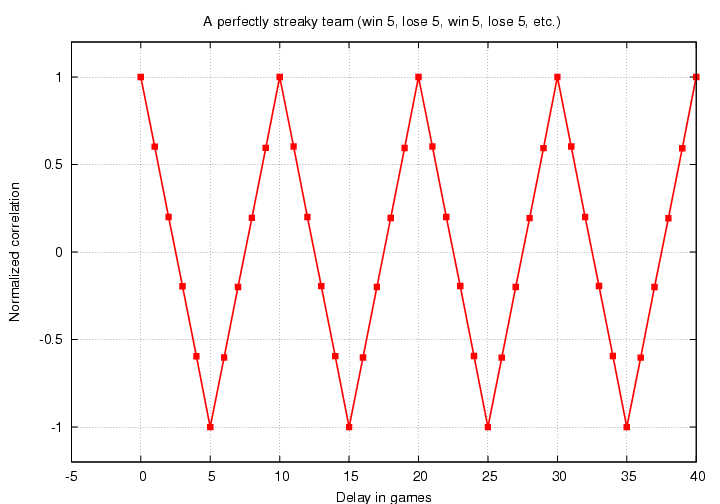
If we look ahead 5 games, we switch from a winning to a losing streak (or vice versa), so the result of game i is always exactly OPPOSITE to game i+5; and so C(5) is exactly -1. But if we look ahead 10 games, we move back into the next winning (or losing) streak, which means the result of that game is always the same as the result of the current game; and so C(10) is exactly +1.
This example is non-sensical; no team is so perfect in its streakiness.
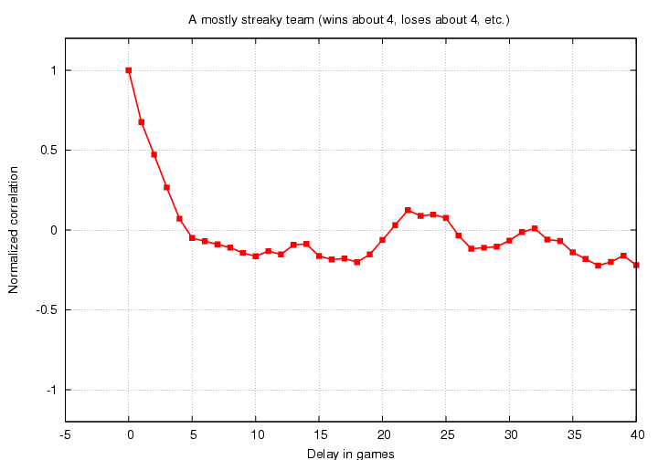
There is a strong positive correlation for offsets of 0-4 games, then a weak negative correlation, then a somewhat random fluctuation for large offsets. This is much more realistic. In real life, we expect that the correlation should become small and random for very large offsets, because there shouldn't be any connection between the game today and the game two months from now.
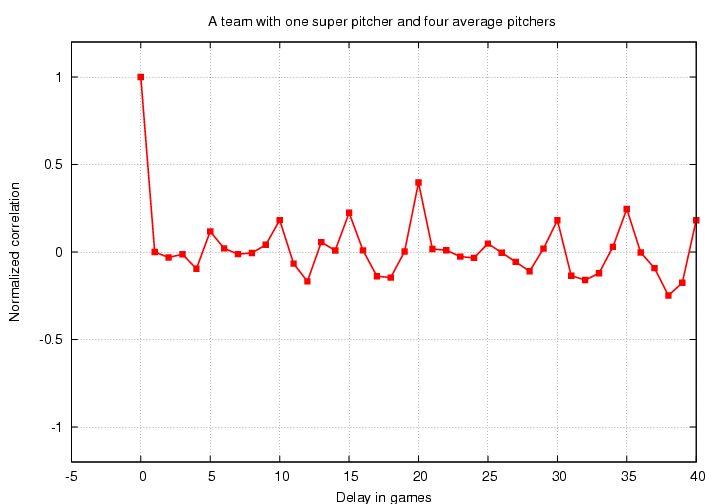
We see peaks in the correlation function for delays divisible by 5: C(5) sticks out in the positive direction, C(10) does too, C(15), and so forth. Note that none of these peaks goes up to a height of 1.0, because the (almost) perfect correlation of Pedro's starts is mixed with the random correlation of each of the average pitchers' starts. The fact that C(20) is higher than rest is just a random fluctuation; if I generate a second season in the same manner, some other peak will be higher.
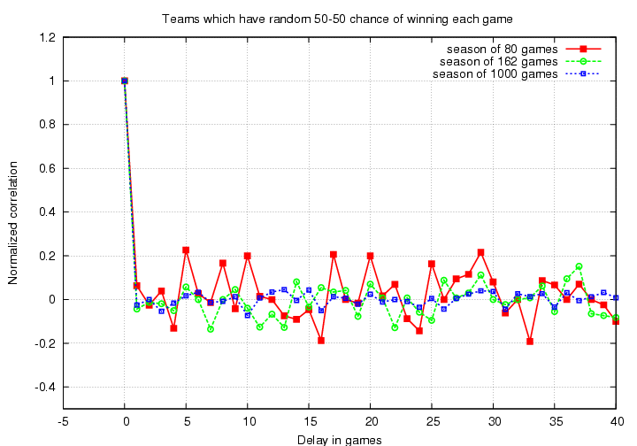
there are small fluctuations around zero. The longer the season -- the more terms we add together to compute the autocorrelation function -- the smaller those fluctuations become. We can estimate the magnitude of the fluctuations σ as

where N is the number of games in the season. We can expect the great majority of the fluctuations to be less than 2*σ in size; for a standard 162-game season, that means most random peaks in the correlation function should be less than +/- 0.16.
Okay, now that we know what to expect, let's take a look at the autocorrelation function of real baseball teams. My sample of the American League contains 594 team-seasons, each of which contains a string of 162 wins and losses.
First, let's look at the autocorrelation function of all these teams put together; I calculated the correlation function for each team individually (making the small adjustments necessary for teams with overall winning or losing records), then added together all the C(1) values, all the C(2) values, and so forth. I also shifted the data slightly to remove a zero-point bias, so that the correlation function at very large delays was forced to zero. Here are the results:

The parallel black lines show the expected 2σ range inside which random variations should lie. It appears to me that there is a significant positive correlation for Δ = 1, and possibly another positive correlation for Δ = 3.
Before we start imagining reasons for the positive correlations, let's double-check by looking at the same analysis applied to a completely random set of numbers. I generated random wins and losses for the same number of team-seasons and ran all those fictional seasons through the same procedures as the real data.
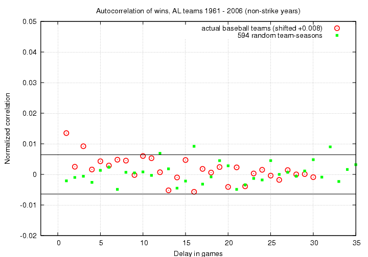
Hmmm. The majority of the random (green) points lie within the expected range of +/- 0.0064; that makes sense. But note that three of the random correlation values do appear outside the boundaries, on the positive side. Two of these three have roughly the same amplitude as the C(3) value of the real data. This suggests to me that the apparent correlation in the real data between game i and i+3 may not be real ...
The only significant non-zero correlation, I would claim, is the one between neighboring games. The correlation function has a value C(1) = 0.0135 ... but just what does that mean, in everyday terms?
To answer that question, I modified my random-season generator slightly so that I could put into it a variable degree of connection between games. Specifically, I first generated a set of pure random numbers with a uniform distribution between 0.0 and 1.0, just as I had before. By setting a threshold at 0.5, and assigning "Wins" to larger values and "Losses" to smaller values, I could create an artificial, random season. Now, however, I tweaked those random values by "smoothing together" adjacent numbers: I added a fraction α of all neighboring values within some range L.

For example, suppose α = 0.10 and L = 1. If games 9, 10 and 11 were originally assigned random values 0.7, 0.4, 0.6 -- meaning "Win", "Loss", "Win" -- then the smoothing procedure would modify the score for game number 10 to be
                                           1    (                     )
      new score  =  original score  +    ------ ( 0.1*0.7  +  0.1*0.6 )
                                          1.2   (                     )

                                           1
                 =       0.4        +    ------ ( 0.13 )
                                          1.2


                 =       0.4        +     0.11


                 =       0.51
Game number 10 would now become a "Win", due to the influence of the games surrounding it. This "smoothing" introduces a correlation between games which are within +/- L of each other. Therefore, it will create significant positive correlation values for values of Δ ≤ L.
I chose a correlation length L = 3 games. I then fiddled around with the value of α until I could very roughly reproduce the observed positive correlation peak at C(1). I stopped when I came this close:
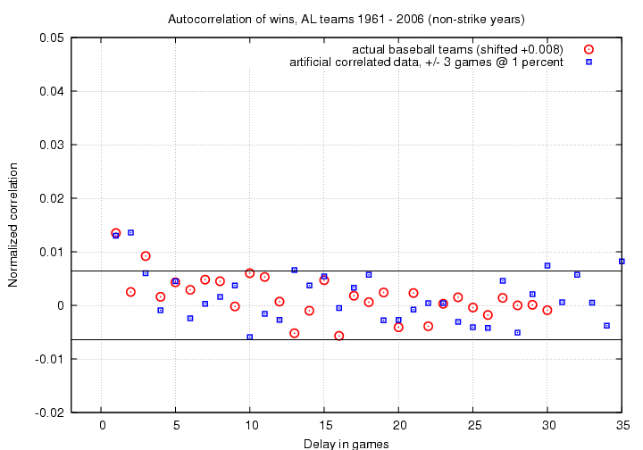
What value of α matched the real data this well? A pretty small one: α = 0.01. In other words, the historical data does suggest that the result of today's game can affect the result of tomorrow's game .... but only to a very small degree. I'm not exactly sure how to put it into words, but something like this is probably close:
If you win today, you are 1 percent more likely than usual to win tomorrow, too; if you lose today, you are 1 percent more likely than usual to lose tomorrow, too.
Time for a very brief bit of speculation: if there really is a weak correlation between neighboring games, what might cause it? I can come up with a number of guesses, but I have no idea which, if any, are correct.
I really ought to perform a similar analysis of other datasets -- the National League, seasons earlier than 1961 -- to see if the same excess correlation at 1 (and 3?) games appears.
 Copyright © Michael Richmond.
This work is licensed under a Creative Commons License.