Revised to use Contextual Runs to predict a team's performance, rather than OPS. You can still read the original version using OPS if you wish.
This question was posed as part of a discussion on the Sons of Sam Horn website . Eric Van asked the question:
What we want to know is whether there's a correlation between standard deviation of the principal hitters, and two things: Actual Runs - Calculated Runs according to EqA, CR, RC or other formula Actual Wins - Pyth Wins IOW, do consistent lineups score more or less runs than expected? Given however many runs they score, do consistent lineups win more or less games than expected?
I will attempt to address the first question: does the actual number of runs scored by a team depend significantly on whether the hitters are relatively uniform in quality, or vary greatly from batter to batter?
For the impatient among you, my conclusion is "No."
The basic data comes from baseball-reference.com's website . I used their list of the "main starting batters" for all American League teams during the period 1997-2006. For example, the 2006 Red Sox are listed like so:
Pos Player              Ag   G   AB    R    H   2B 3B  HR  RBI  BB  SO   BA    OBP   SLG  SB  CS  GDP HBP  SH  SF IBB  OPS+
---+-------------------+--+----+----+----+----+---+--+---+----+---+----+-----+-----+-----+---+---+---+---+---+---+---+----+
C  #Jason Varitek       34  103  365   46   87  19  2  12   55  46   87  .238  .325  .400   1   2  10   2   1   2   7   85
1B  Kevin Youkilis      27  147  569  100  159  42  2  13   72  91  120  .279  .381  .429   5   2  12   9   0  11   0  108
2B  Mark Loretta        34  155  635   75  181  33  0   5   59  49   63  .285  .345  .361   4   1  16  12   2   5   1   82
3B  Mike Lowell         32  153  573   79  163  47  1  20   80  47   61  .284  .339  .475   2   2  22   4   0   7   5  106
SS  Alex Gonzalez       29  111  388   48   99  24  2   9   50  22   67  .255  .299  .397   1   0   6   5   7   7   1   77
LF  Manny Ramirez       34  130  449   79  144  27  1  35  102 100  102  .321  .439  .619   0   1  13   1   0   8  16  168
CF #Coco Crisp          26  105  413   58  109  22  2   8   36  31   67  .264  .317  .385  22   4   5   1   7   0   1   80
RF *Trot Nixon          32  114  381   59  102  24  0   8   52  60   56  .268  .373  .394   0   2  10   7   0   5   1   98
DH *David Ortiz         30  151  558  115  160  29  2  54  137 119  117  .287  .413  .636   1   0  12   4   0   5  23  164
---+-------------------+--+----+----+----+----+---+--+---+----+---+----+-----+-----+-----+---+---+---+---+---+---+---+----+
I also grabbed the overall team stats, using all players, for each team.
By the way, the most time-consuming portion of this work was dealing with the changing name of the Angels team: they went from the California Angels to the Anaheim Angels to the Los Angeles Angels during this brief span. Sigh.
I will use simple OPS, defined as the sum of On-base-Percentage (OBP) and Slugging Percentage (SLG), as a measure of the quality of a batter. If batters have similar OPS, I judge them to be similar; if their OPS values differ greatly, I judge the hitters to be significantly different in quality.
In order to predict the performance of a team, I'll use a slightly modified version of Contextual Runs (CR).
Since my sources didn't list LOB, I set it to zero; sorry! I also scaled the result of the calculation by a constant factor so that, on average over the period of the study, the prediction was equal to the actual number of runs; that happened when I multiplied the CR value by 2.03.
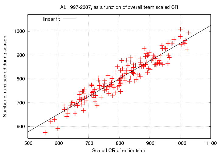
So, if we determine the linear relationship between my "scaled CR" value and the actual number of runs scored, we find:

The linear fit is
     Runs = 204.6  +  0.745*(scaled CR)

                scatter from fit = 28 runs
                uncertainty in slope = +/- 0.040 runs/(scaled CR)
                correlation coefficent  r = 0.943
Those of you who read the earlier version will note that scaled CR does indeed predict actual runs scored better than OPS.
It's clear from the graph that some teams score more runs than this model predicts, and other score fewer. The question is -- are those differences from the basic model due to the inhomogeneity of the lineup? Suppose that they were; then we might expect lineups with a mixture of great and terrible hitters to score more runs (or fewer runs) than the model predicts. In that case, most of the points lying above (or below) the line would represent teams with a mixture of good and bad hitters.
One way to test this idea is to subtract from a team's ACTUAL number of runs scored the number of runs predicted based on its scaled CR. We can then plot this residual, in the sense
residual = (actual runs scored) - (linear model using scaled CR)as a function of the inhomogeneity of the main starting 9 batters. If the hypothesis is correct, we will see a correlation in the graph.
To quantify the inhomogeneity of the main 9 starters, I simply computed the standard deviation from their mean OPS during the season. In other words, using only the stats of the main 9 starting batters, I computed
                    sum ( OPS of each batter)
      mean OPS  =  ---------------------------
                             9
                                                2                 2
                      (  sum(OPS of each batter)   -  9*(mean OPS)    )
     stdev OPS  = sqrt( --------------------------------------------- )
                      (                   (9 - 1)                     )
For example, in the case of the 2006 Red Sox, the main 9 starters had a mean OPS = 0.814 and a standard deviation of 0.143. By comparison, the overall team OPS was 0.786, so the bench players were (as a group) rightly kept on the bench.
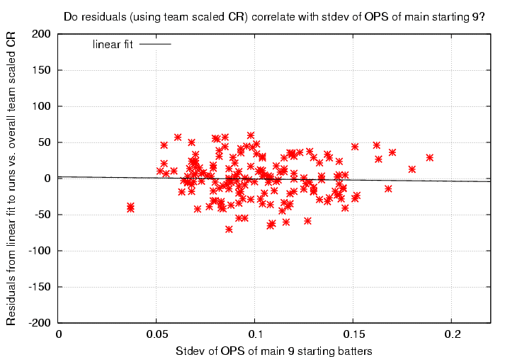
So -- do the residuals in runs scored over a season correlate with the inhomogeneity of the main 9 batters?

In a word, no: there is no correlation here. A formal unweighted linear fit to the residuals as a function of stdev of starting 9's OPS is
       residuals  =  2.334  - 23.711*(stdev OPS of starting 9)

                 scatter = 28 runs
                 uncertainty in slope = +/- 149 runs/(stdev OPS)
                 correlation coefficient  r = -0.024
For the curious, I include here a few "top 10" and "bottom 10" lists generated during the course of this study. First, let's pick the teams which deviated most in a bad way -- underperformed, in other words -- from the linear model using scaled CR.
#
#                          mean  stdev                mean                                  residual
#---------------------------------------------------------------------------------------------------
 1996  MIN  starters ops  0.802  0.087  overall ops  0.778  runs   877  scaled cr   808.0    -70.3
 2001  SEA  starters ops  0.810  0.108  overall ops  0.805  runs   927  scaled cr   881.5    -65.5
 1997  NYY  starters ops  0.813  0.109  overall ops  0.798  runs   891  scaled cr   837.8    -62.1
 2000  KCR  starters ops  0.793  0.116  overall ops  0.773  runs   879  scaled cr   823.9    -60.4
 1999  CLE  starters ops  0.873  0.127  overall ops  0.839  runs  1009  scaled cr  1000.7    -58.7
 1998  OAK  starters ops  0.747  0.092  overall ops  0.731  runs   804  scaled cr   730.7    -54.9
 2002  ANA  starters ops  0.789  0.095  overall ops  0.774  runs   851  scaled cr   793.9    -54.8
 2003  SEA  starters ops  0.757  0.114  overall ops  0.754  runs   795  scaled cr   732.1    -44.8
 1996  NYY  starters ops  0.808  0.071  overall ops  0.796  runs   871  scaled cr   837.5    -42.3
 2005  TOR  starters ops  0.744  0.037  overall ops  0.738  runs   775  scaled cr   708.8    -42.2
I see no patterns here.
Let's look at the teams which overperformed the most relative to the prediction of their overall OPS:
#                          mean  stdev                mean                                  residual
#---------------------------------------------------------------------------------------------------
 2002  DET  starters ops  0.691  0.096  overall ops  0.679  runs   575  overall cr   556.9     44.6
 2000  TOR  starters ops  0.832  0.162  overall ops  0.810  runs   861  overall cr   942.5     46.0
 2002  BAL  starters ops  0.717  0.054  overall ops  0.712  runs   667  overall cr   682.4     46.1
 2003  CHW  starters ops  0.796  0.101  overall ops  0.777  runs   791  overall cr   850.9     47.7
 2005  CHW  starters ops  0.768  0.068  overall ops  0.747  runs   741  overall cr   786.8     49.9
 2005  TEX  starters ops  0.815  0.081  overall ops  0.797  runs   865  overall cr   959.4     54.5
 2005  BAL  starters ops  0.784  0.080  overall ops  0.761  runs   729  overall cr   778.3     55.6
 1999  DET  starters ops  0.792  0.061  overall ops  0.761  runs   747  overall cr   804.5     57.1
 2006  TBD  starters ops  0.763  0.085  overall ops  0.734  runs   689  overall cr   726.8     57.2
 2003  DET  starters ops  0.711  0.098  overall ops  0.675  runs   591  overall cr   598.5     59.6
Hmmm. Detroit appears 3 times, Baltimore and the White Sox twice. This repetition might possibly suggest that there is some feature of these teams which causes them to do better than scaled CR would predict, but it could very well be chance.