Contents
This talk describes the results of a very large effort, by a team of tens of astronomers and engineers, from many different institutions. I have played just a very small role in these projects; one might describe me as a very interested bystander. My contributions have been connected to Mamoru Doi and Tomoki Morokuma, two astronomers at the Institute of Astronomy in Tokyo. The final sections of this talk describe two papers written by Morokuma-san (and others) which appeared recently on astro-ph.
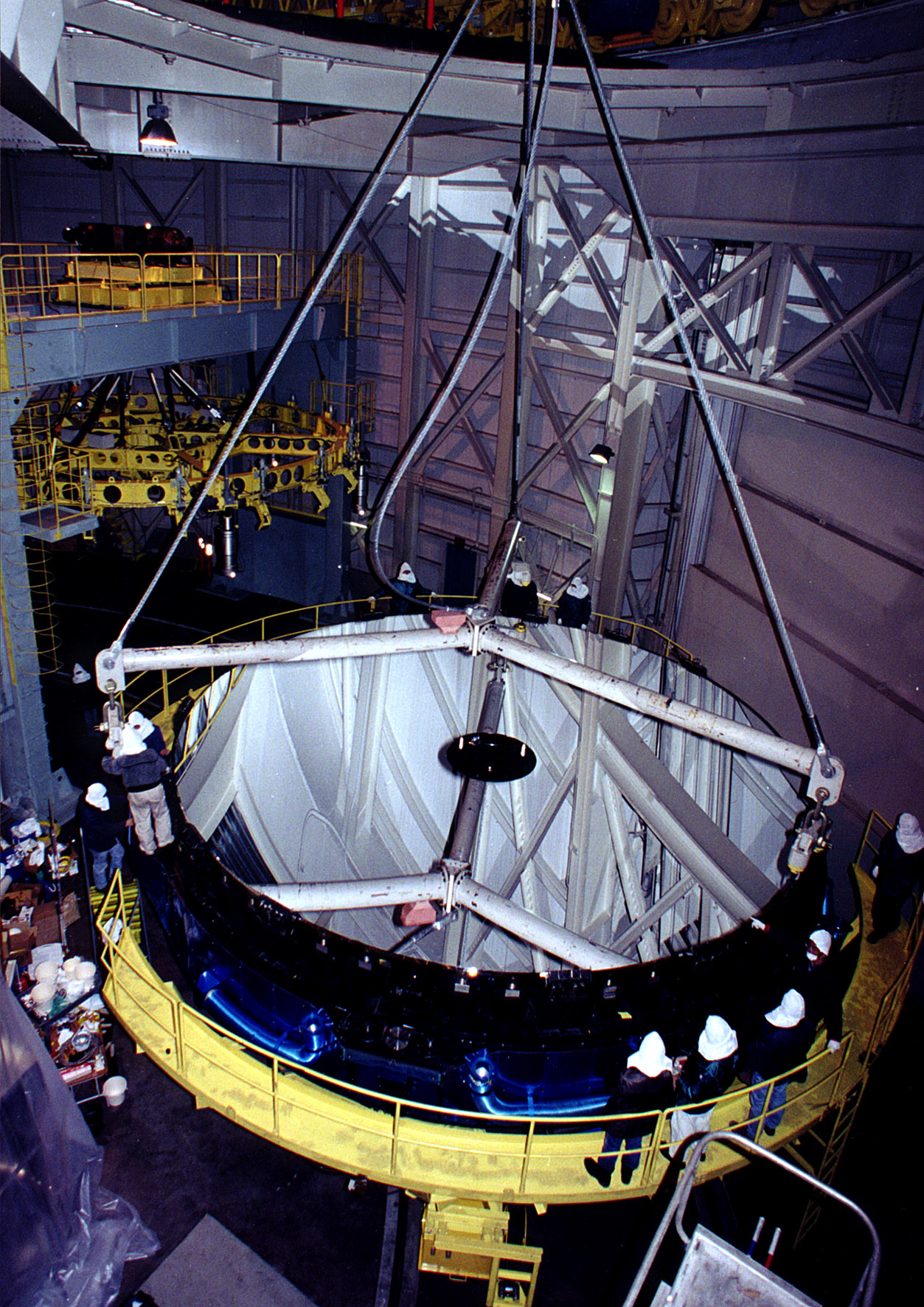
The Subaru telescope is one of the largest optical telescopes in the world. It has a primary mirror made from a single slab of glass 8.2 meters in diameter:
The telescope sits within an enclosure near the peak of Mauna Kea, 4100 meters above sea level.
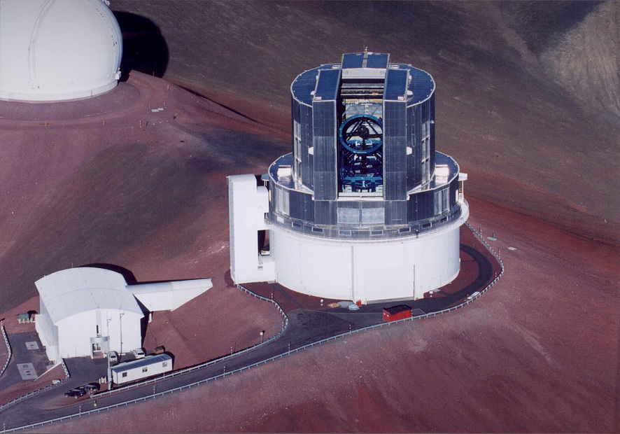
Image courtesy of NAOJ
The instrument used for much of the work I will describe is called Suprime-Cam . This camera contains 10 large CCDs arranged in a rectangular block; the picture below shows only 6 of them. Each CCD is 2048x4096 pixels, so a single image taken by the entire camera contains roughly 84 million pixels. Since each pixel is read out into a 16-bit number, a single raw image fills about 168 Megabytes of memory.
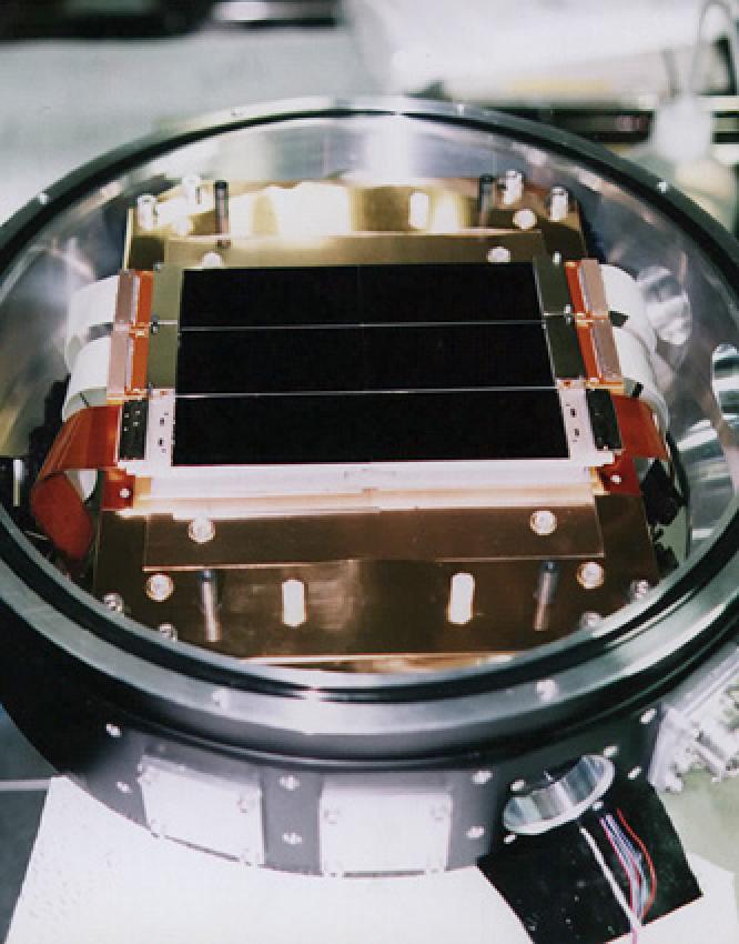
Suprime-Cam, mounted on Subaru, covers a very wide area of the sky , compared to many other cameras mounted on big telescopes. The field of view is 37x27 arcminutes, or about 0.28 square degrees. For comparison, the largest field of view available from the ACS camera aboard HST is only 3.4x3.4 arcminutes, or 0.003 square degrees. (And, at the moment, this portion of ACS is not working).
So, together, the Subaru telescope and the Suprime-Cam instrument provide images which are very wide and very deep. In a one-hour exposure, the combination reaches a limiting magnitude of roughly 27, depending slightly on the passband.
The Subaru/XMM-Newton Deep Survey (or SXDS for short) is one small region of sky which has been chosen for intensive study. It lies near the celestial equator and not far from the southern galactic pole at coordinates
02h 18m -05d 00' (J2000)
marked by the golden circle in the chart below.
Since this area is far from the plane of the Milky Way (galactic latitude -60 degrees), when we look at it, we avoid most of the dust and gas in our own galaxy. We can therefore see faint objects which lie very very far away. This region also is equally visible to instruments in the northern and southern hemispheres, allowing all observatories to study it.
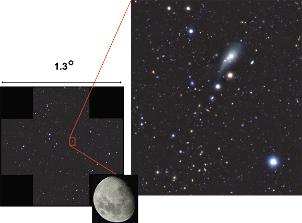
This region of the sky has also been chosen for intensive study by telescopes using other wavelengths of light.
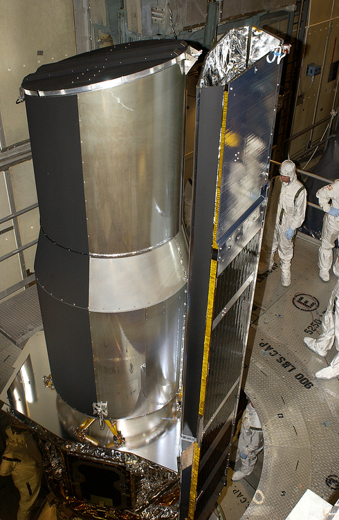
The XMM-Newton space telescope was launched by the ESA in 1999. It is one of the largest X-ray telescopes in orbit.

It has taken very long exposures of the SXDS field. Because its field of view is a bit smaller than that of Suprime-Cam, the XMM telescope took a series of 5 images in the form of a cross to capture the entire area. The image below is color-coded so that high-energy photons are blue, low-energy photons are red.
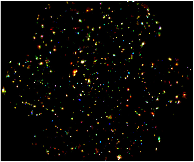
has also taken a set of infrared images of this region. Unfortunately, I don't have a nice composite image to show you ...
The Subaru telescope has visited this field several times from 2002 to the present. The analysis below is restricted to measurements made over a three-year period, 2002 to 2005. Most of the images were taken in the i-band, with typical exposure times of 1 hour and limiting magnitudes of about 26 for point sources. The total area was very roughly one square degree.
The data were subjected to an image-subtraction technique, in which individual images are convolved to match a template, and then the template is subtracted from the image. Over the course of the project, a total of 1153 objects -- about 5 percent of all detected sources -- were determined to vary significantly. Each variable object was matched, if possible, to a "host", using a very deep stack of images from several years.
The X-ray and infrared measurements were made at only a single epoch, so there is no information on the variation of flux at these wavelengths. However, each of the objects which varied in the optical was matched, if possible, to sources in the X-ray and IR images. The IR data at the shortest wavelength, 3.6 microns, was used to help classify the variable objects.
In the figures above, the large and dark symbols indicate stars, while the small, light grey symbols indicate non-stars. Note that only a small fraction, about 10 percent, of the variable objects are likely to be stellar.
The non-stellar sources could be either SNe immersed in a host galaxy, or AGN. One can distinguish between these two possibilities in several ways:
In each case, the light of the variable component is mixed with the light of the host. Our ability to identify variable objects securely drops to zero at around i = 24.5 .
Look at the left-most column in the figure below. Roughly two percent of all sources detected between 20.5 < i < 22.0 are time-varying AGN, while roughly one percent are SNe. If one computes the density of sources per square degree at these magnitudes, one finds roughly
     Type                Number per square degree
    ----------------------------------------------
     variable star             120

     supernova                 490

     AGN                       580
    ----------------------------------------------
After matching these optically variable objects to the sources in the deep X-ray images, one finds that roughly 36 percent of all X-ray sources turn out to vary in the optical; the fraction is slightly higher if one looks at the more secure measurements of bright optical objects.
Now, there are a total of 211 AGN which show optical variations in the portion of the SXDS which was observed by the XMM satellite. There are 327 X-ray sources detected in this same region. What can we learn by comparing these two samples, selected by entirely different means?
One can divide the AGN in this field into three categories:
  name      X-rays?      optical?    optically variable?
----------------------------------------------------------
   XA         yes          yes            no

  XVA         yes          yes           yes

   VA          no          yes           yes
----------------------------------------------------------
Consider the "VA" category first: AGN which do not appear in the X-ray images. Is there any property of these sources in the optical which also separates them from the X-ray "loud" AGN? Yes, there is: if we look at the ratio of
        flux from varying optical component
       -------------------------------------
        flux from constant optical component
we find that most of the "VA" sources have relatively small ratios, while the X-ray-detected objects have large ratios.
These distributions are clearly different. This suggests that we might be seeing two populations of AGN:
Suppose that we concentrate on properties of the X-rays measured from X-ray sources. Let's look at the hardness ratios of the AGN which showed no optical variation, and those which did show optical variation. The hardness ratio HR2 is defined to be large positive for "hard" sources with mostly high-energy photons, and negative for "soft" sources with mostly low-energy photons.
There's a clear difference here:
What might this tell us? One interpretation is that the presence of optical variability depends on the orientation of the AGN:
In other words, using deep optical images to find variable objects can be an efficient way to select Type 1 AGN. Note that some of the AGN in the optical sample, those denoted "VA", do not appear at all in deep X-ray images.