 Copyright © Michael Richmond.
This work is licensed under a Creative Commons License.
Copyright © Michael Richmond.
This work is licensed under a Creative Commons License.
There are several different techniques for acquiring spectra of exoplanets and their atmospheres. In brief, they are
This is the really interesting option, in my opinion. As a planet passes in front of its star, oodles of light from the star fly through the atmosphere, probing it thoroughly at a range of depths.
One of the problems is that only a tiny fraction of the star's light goes through the planet's atmosphere.
![]()
   Q:  Write an equation which expresses the fraction of
             observed light transmitted by the
             planet's atmosphere.


   Q:  For a typical Hot Jupiter, what is this fraction?


   Q:  For an Earth-sized planet, what is this fraction?
The expected signal is very small (as is always the case with exoplanet science). That means that one must perform very careful calibration and data reduction. Fortunately, since a transit only lasts a few hours, it will often be possible to acquire the in-transit vs. out-of-transit comparison data during a single session on a single night.
Let's look at a Good Case: Spectrally resolved detection of sodium in the atmosphere of HD189733b with the HARPS spectrograph by Wyttenbach et al. (2015). Fig 1 from their paper shows the importance of removing features caused by the Earth's atmosphere. On their "Night 3", they had to perform two rounds of corrections because the properties of the air had changed from one night to the next.
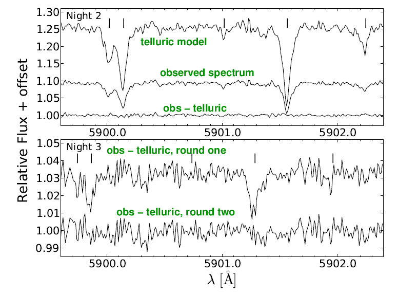
Fig 1 modified from
Wyttenbach et al., arXiv 1503.05581v1
However, the payoff is great: after performing all the calibrations, and co-adding spectra taken over three nights (each night including some inside and outside of the transit), the authors find a clear detection of sodium absorption lines due to the planet's atmosphere:
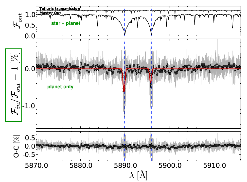
Fig 2 modified from
Wyttenbach et al., arXiv 1503.05581v1
Note the change in the vertical scale from the top panel to the bottom panel!
This group used the high-resolution HARPS spectrograph on the ESO 3.6-meter telescope at La Silla, Chile. Compare their results to earlier measurements (Huitson et al., MNRAS 422, 2477 (2012) made with the 2.4-meter HST and STIS spectrograph. Big, special-purpose, high-resolution spectrographs can yield excellent results.
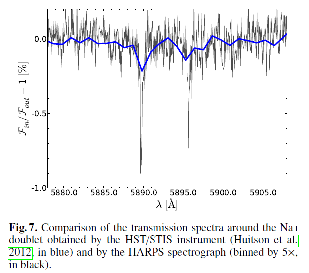
Fig 7 from
Wyttenbach et al., arXiv 1503.05581v1
Let's take a moment to review the observations. This star, HD 189733, is roughly V = 7.6. The authors spent three nights observing the star -- measuring one transit each night -- and then combined their results. They DID detect a feature due to the planet's atmosphere, clearly. Do the numbers add up?
   Recall that a V = 0 star produces about 10^6 photons
             per square cm. per second in V-band.
             The authors used a telescope with radius 180 cm.

     Q:  How many photons should they have collected per second?


     Q:  In order to see a feature with fractional depth approx = 10^(-4),
             how many photons must they collect?


     Q:  How long should they need to expose?


     Q:  How long _did_ they expose?


     Q:  Why the difference?  Have we forgotten something?
But the previous example was one of the best detections of an atmospheric feature I've seen. More typical, perhaps, is the following, taken from Sedaghati et al., A&A, 576, L11 (2015) . They used the FORS spectrograph on the 8-m VLT to observe the planet WASP-19b as it moved in front of its star.
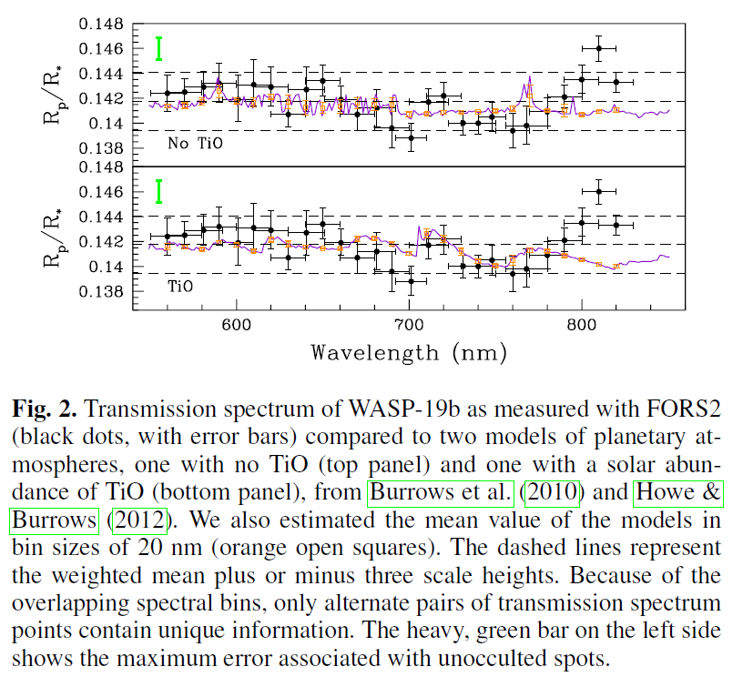
Fig 2 from
Sedaghati et al., A&A, 576, L11 (2015) .
Q: Do you conclude that this planet has TiO in its atmosphere?
And in some cases, it turns out that we seem to move BACKWARDS the harder we try. Consider the case of Hoeijmakers et al., A&A 575, 20 (2015). They tried to measure absorption by TiO in the atmosphere of HD 209458b during a transit, using the 8.2-m Subaru telescope and its High Dispersion Spectrograph between 5500 and 6700 Angstroms.
First, they found no positive result when they compared their spectrum of the planet's atmosphere to a model spectrum with TiO.
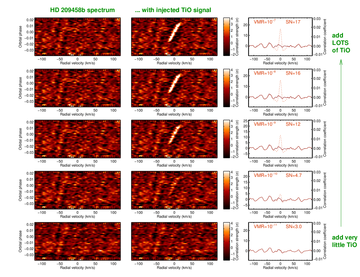
Figure 5 modified from
Hoeijmakers et al., A&A 575, 20 (2015).
But the situation is worse -- when they used the same equipment to observe Barnard's Star, which is KNOWN to have plenty of TiO in its very cool stellar photosphere, they could not reliably detect the molecular features!
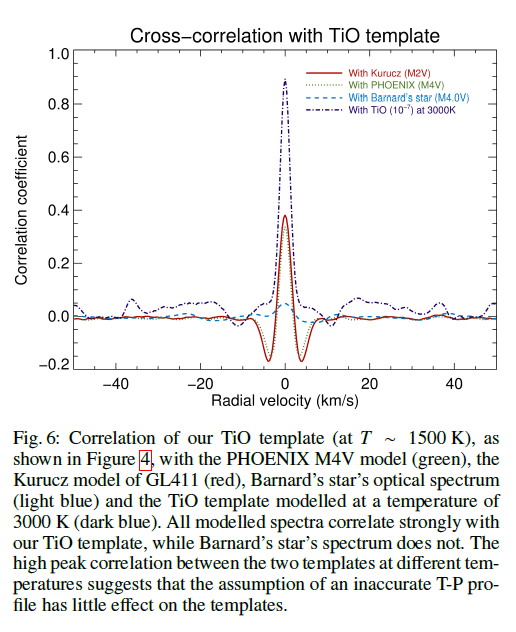
Figure 6 modified from
Hoeijmakers et al., A&A 575, 20 (2015).
The authors tracked the problem down to an issue with the line lists for TiO. Apparently, the measured (or calculated?) wavelengths of the many, many, many transitions of this molecule may contain a number of inaccuracies, enough to confuse the correlation procedures.

Text taken from
Hoeijmakers et al., A&A 575, 20 (2015).
As we try to study exoplanetary atmospheres in more detail, we learn that we need to learn more.
In fact, in some cases, we discover more about the host star than the planet which orbits it. Consider the case of WASP-52b. The transit light curves show a somewhat ... uneven shape.
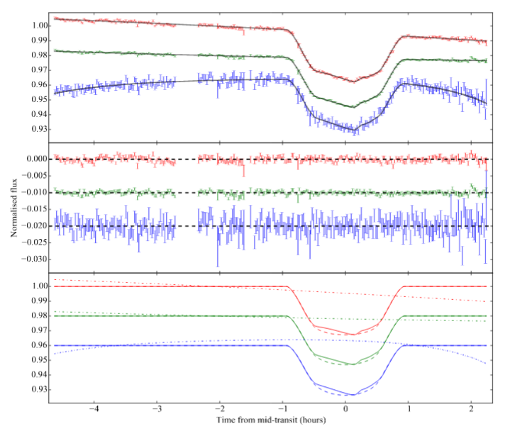
Figure 2 taken from
Kirk et al., MNRAS 463, 2922 (2016)
The authors suggest that the planet moved over EITHER
In order to measure the size of the planet properly, one must know accurately the amount of light behind it. And if one does not know EXACTLY how light was distributed on the stellar surface, then one might make an error in calculating the tiny fraction of that light blocked by the planet at different wavelengths.
Which ... could make a big difference in the properties of the atmosphere which could be derived:
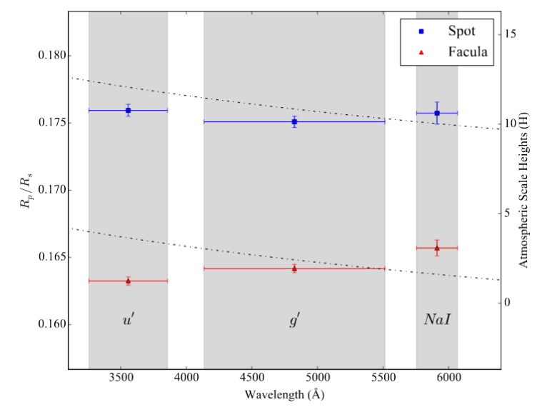
Figure 6 taken from
Kirk et al., MNRAS 463, 2922 (2016)
This transmission spectroscopy is a very, very tricky business.
The idea here is to separate the reflected light of the planet from that of the host star, and analyze the spectrum of that reflected light.
This is going to be difficult -- very difficult. The problem is that one must do several difficult things, all at once:
The real problem is the last one: there just aren't many photons coming from the planet, so there's very little signal-to-noise left after one has split the light with a spectrograph.
So, perhaps a more likely approach in the near future will be photometry of the reflected light, rather than spectroscopy. You can think of photometry as "very low-resolution spectroscopy", using bins which are hundreds or thousands of Angstroms wide, instead of the usual fractions of an Angstrom.
It turns out that there are some reasonably clear clues to the properties of an exoplanet and its atmosphere which may be detected with optical photometry. Below are spectra of the planets in our Solar System in the visible range:
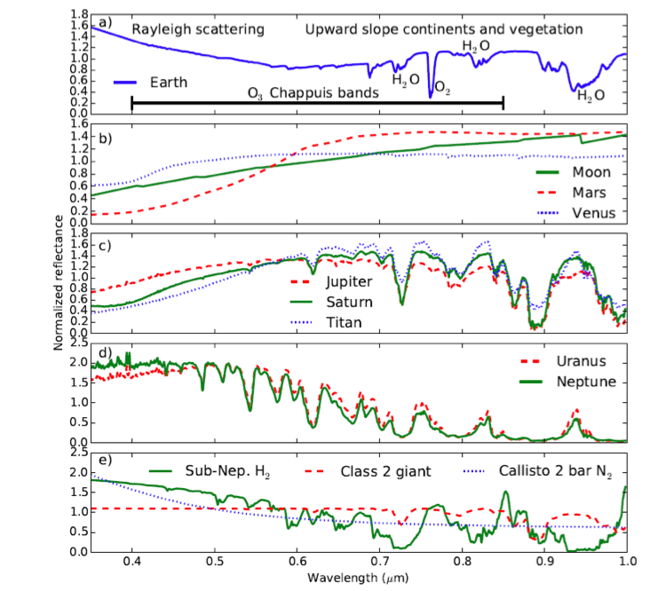
Figure 1 taken from
Krissansen-Totten et al., ApJ 817, 31 (2016)
Note that the Earth reflects light strongly in the blue part of the optical spectrum -- but, of course, you already know that.
That blue light is due to Rayleigh scattering of incoming sunlight by the molecules within the Earth's atmosphere. We have a pretty dense atmosphere, so there's lots of scattering, so lots of blue light goes bouncing off in all directions.
Figure 1 taken from
Krissansen-Totten et al., ApJ 817, 31 (2016)
It turns out that ozone (O3) absorbs light strongly in the middle of the optical -- green and yellow -- and so creates a bit of a dip in the Earth's spectrum.
Rocks tend to reflect more light in the red. Chlorophyll absorbs light strongly in the yellow, orange and red, but then stops absorbing around a wavelength of 7000 Angstroms, leading to an increase in reflected light. This change is sometimes called the "Red Edge". Together, these two effects increase the brightness of the Earth in the near-infrared.
So, the Earth's reflection changes from bright in blue, to faint in yellow, to bright in red.
Figure 1 taken from
Krissansen-Totten et al., ApJ 817, 31 (2016)
Note that other planets show very different patterns.
The bottom line is that if one were to take pictures in just three broad passbands -- "red", "green", and "blue" -- one could separate an Earth-like planet from most other varieties.
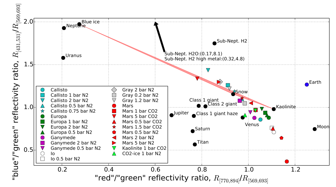
Figure 2 taken from
Krissansen-Totten et al., ApJ 817, 31 (2016)
Earth's unusual optical spectrum -- brighter at both ends than in the middle -- causes it to fall in the upper-right portion of this "color-color diagram".
If we could take even mediocre images of exoplanets through broad optical filters, we could use diagrams like this to classify them into very rough categories.
Consider a planet orbiting close to its star. If the planet is hot, either from its own internal heat sources or due to the stellar radiation, it will emit light as a blackbody. How bright will it appear compared to the star?
Well, if we treat both the star and planet as blackbodies, the ratio of their fluxes will be
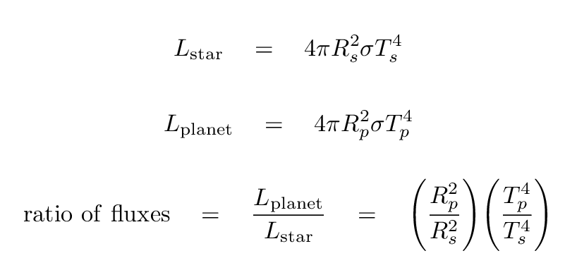
   Q:  Compute this ratio for a typical Hot Jupiter
             around a sun-like star.


   Q:  Compute this ratio for an Earth-like planet
             in an Earth-like orbit
             around a sun-like star.
It's clear, once again, that detecting even the biggest, brightest planets will be no easy matter; and that detecting Earth-like planets is, in the words of Brother Maynard, Right Out!
Still, let's look at an example of this technique in action. You'll see that to call this "spectroscopy" is a bit of a stretch; it's really just photometry. It might be better to call this thermal "extremely low-resolution spectroscopy".
Our example is a study of the planet around HAT-2-P by Lewis et al. They compare Spitzer measurements of this planet in the near-IR to a number of atmospheric models. The planet is big (8.9 times the mass and 1.1 times the radius of Jupiter) and close (period = 5.6 days, semi-major axis = 0.07 AU) to its host star; in other words, a pretty standard Hot Jupiter.
But note that this system is NOT as simple as we often pretend. In particular, the orbit of the planet is not circular.
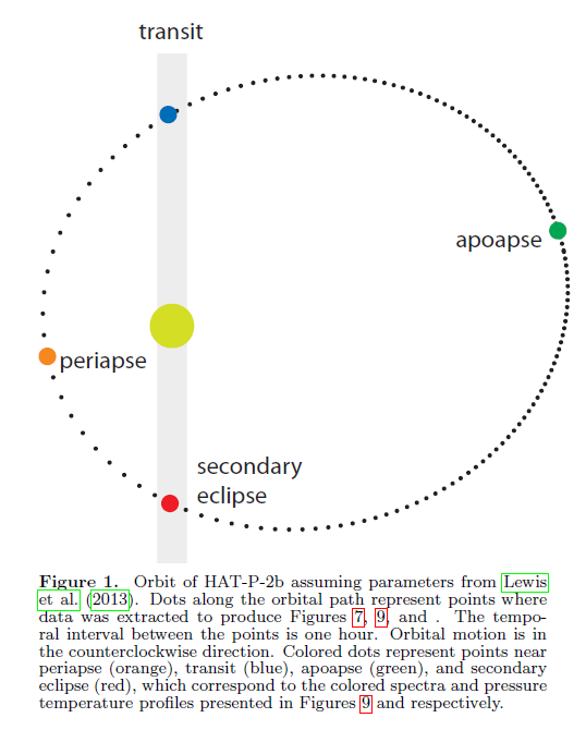
Fig 1 taken from
Lewis et al., ApJ 795, 150 (2014)
This change in distance from the host star means a big change in the effective temperature of the planet over the course of its orbit. Remember that the orbital period is just 5.6 days.
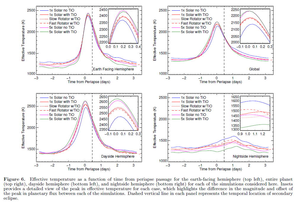
Fig 6 taken from
Lewis et al., ApJ 795, 150 (2014)
So, what do the authors actually measure with Spitzer? Their measurements are shown in the figures below as the black symbols; all the other colored symbols represent the predictions of various models.

Among the conclusions of this study are:
   Q:  How many existing instruments can observe this system
           at wavelengths longer than 4.5 microns?
Copyright © Michael Richmond.
This work is licensed under a Creative Commons License.