
I warned you last time that simulating time-dependent heat conduction might be tricky, due to numerical instabilities. What did I mean by that? Let's find out today by following the operations of a computer which is implementing the equations we derived last time, step by step.
The situation is this: a metal rod of length L = 2 m is initial at temperture T = 0. Then, at time t = 0 sec we attach to the left end a source of heat at a fixed temperature TL = 100 K, and to the right end of the rod a source of heat at a fixed temperature of TR = 10 K. The coefficient of thermal diffusivity of this metal is k = 10-4 m^2/s. What happens next?
Well, that depends on exactly how we choose to simulate the physical situation. Suppose we try this combination of parameters:
Let's focus on the left-hand end of the rod, connected to the source at fixed temperature TL = 100 K.
                                                d2T        T(i+1) + T(i-1) - 2T(i)                          d2T
Time           Temperature                      ---- =    -------------------------                     k  -----  dt
                                                dx2                dx*dx                                    dx2


        100    0    0    0    0    0    0       X   10000    0     0     0     0     0       X    100    0    0    0    0    0
  0     ____ ____ ____ ____ ____ ____ ____     ____ _____ _____ _____ _____ _____ _____     ____ ____ ____ ____ ____ ____ ____

        x=0   0.1  0.2  0.3  0.4  0.5  0.6     x=0   0.1   0.2   0.3   0.4   0.5   0.6      x=0   0.1  0.2  0.3  0.4  0.5  0.6


100     ____ ____ ____ ____ ____ ____ ____     ____ _____ _____ _____ _____ _____ _____     ____ ____ ____ ____ ____ ____ ____


200     ____ ____ ____ ____ ____ ____ ____     ____ _____ _____ _____ _____ _____ _____     ____ ____ ____ ____ ____ ____ ____


300     ____ ____ ____ ____ ____ ____ ____     ____ _____ _____ _____ _____ _____ _____     ____ ____ ____ ____ ____ ____ ____


400     ____ ____ ____ ____ ____ ____ ____     ____ _____ _____ _____ _____ _____ _____     ____ ____ ____ ____ ____ ____ ____
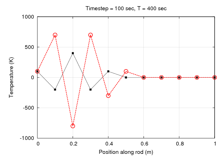
That doesn't look very good, does it? Let's watch the evolution of this simulation graphically:
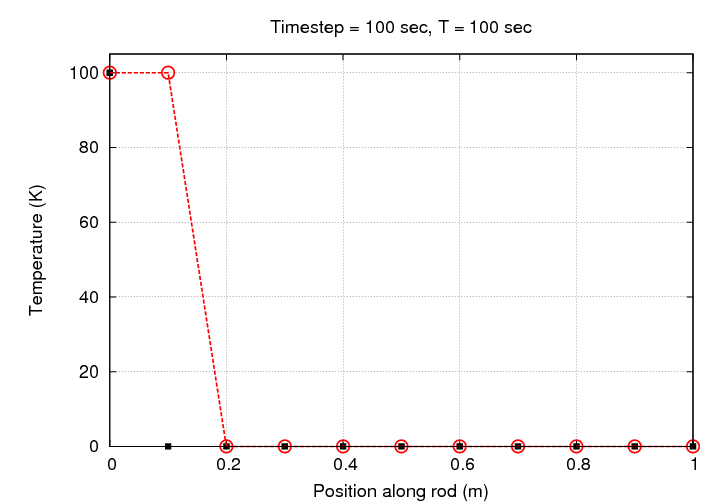
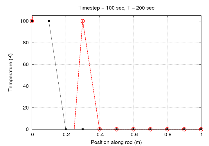
Hey! The temperature at some locations has exceeded our initial range of 0 - 100 Kelvin. In order to see all the values in our numerical array, we need to expand the range. All the following graphs will use the same, much larger range.
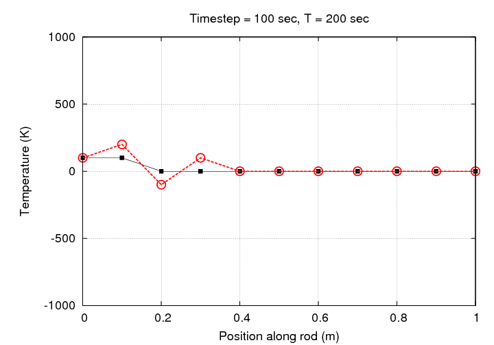
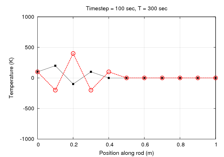
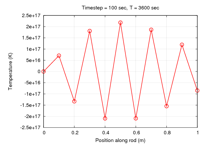
If we let this simulation run for one hour, we end up with baloney; exceedingly bogus baloney, at that.
Look at your worksheet. Can you explain what's going on in this simulation to cause the instability?
How can we avoid that kind of behavior? The answer is to decrease the size of the "steps" in our simulation. We can decrease the steps in time, or the steps in position, or both.
For example, let's cut in half the size of the steps in time:
Again, let's focus on the left-hand end of the rod, connected to the source at fixed temperature TL = 100 K.
                                                d2T        T(i+1) + T(i-1) - 2T(i)                          d2T
Time           Temperature                      ---- =    -------------------------                     k  -----  dt
                                                dx2                dx*dx                                    dx2


        100    0    0    0    0    0    0       X   10000    0     0     0     0     0       X     50    0    0    0    0    0
  0     ____ ____ ____ ____ ____ ____ ____     ____ _____ _____ _____ _____ _____ _____     ____ ____ ____ ____ ____ ____ ____

        x=0   0.1  0.2  0.3  0.4  0.5  0.6     x=0   0.1   0.2   0.3   0.4   0.5   0.6      x=0   0.1  0.2  0.3  0.4  0.5  0.6


        100                                     X                                            X
 50     ____ ____ ____ ____ ____ ____ ____     ____ _____ _____ _____ _____ _____ _____     ____ ____ ____ ____ ____ ____ ____


        100                                     X                                            X
100     ____ ____ ____ ____ ____ ____ ____     ____ _____ _____ _____ _____ _____ _____     ____ ____ ____ ____ ____ ____ ____


        100                                     X                                            X
150     ____ ____ ____ ____ ____ ____ ____     ____ _____ _____ _____ _____ _____ _____     ____ ____ ____ ____ ____ ____ ____


        100                                     X                                            X
200     ____ ____ ____ ____ ____ ____ ____     ____ _____ _____ _____ _____ _____ _____     ____ ____ ____ ____ ____ ____ ____


        100                                     X                                            X
250     ____ ____ ____ ____ ____ ____ ____     ____ _____ _____ _____ _____ _____ _____     ____ ____ ____ ____ ____ ____ ____


        100                                     X                                            X
300     ____ ____ ____ ____ ____ ____ ____     ____ _____ _____ _____ _____ _____ _____     ____ ____ ____ ____ ____ ____ ____
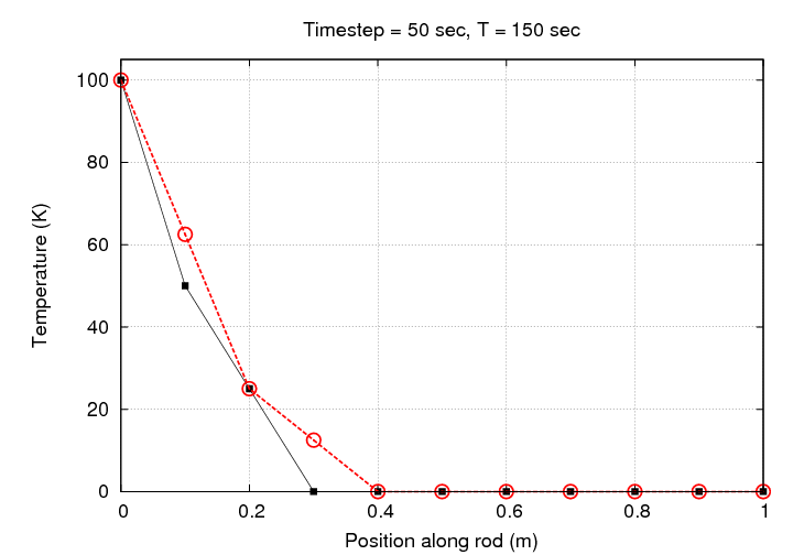
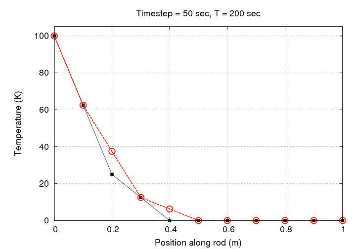
That looks much better, doesn't it? Let's watch the evolution of this simulation graphically:
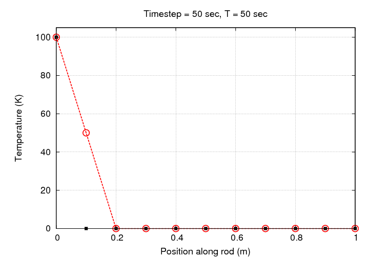
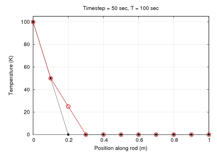
Notice that there's no need to change the scale in this case: all the simulated temperatures fall within the initial range of 0 - 100 Kelvin.
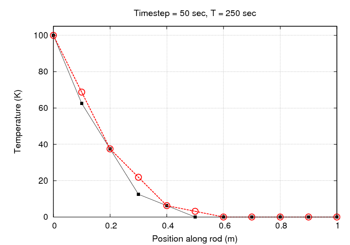
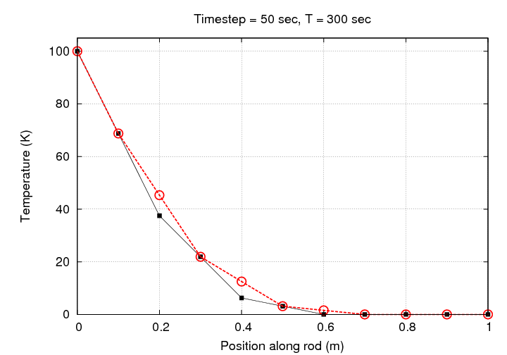
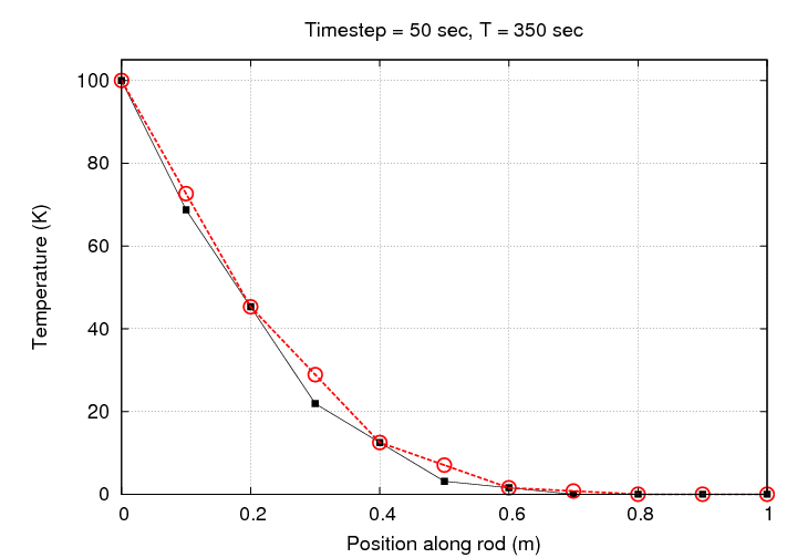
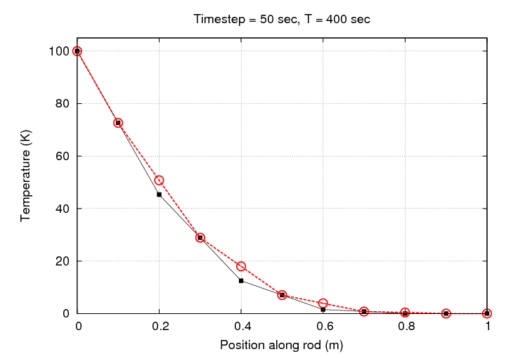
If we let this simulation run for one hour, we end up with a rather nice result:
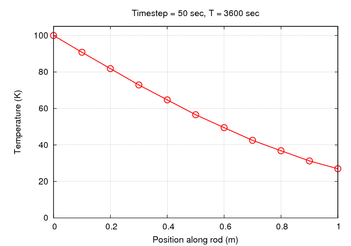
Look at your worksheet. Can you explain what's going on in this simulation to AVOID the instability?
It turns out that one condition for stability in this time-dependent solution is pretty simple: the combination of coefficient of diffusivity k, time-step dt and position-step dx must satisfy
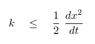
This is necessary, but not sufficient: it's possible that under some circumstances, even if the condition above is true, the numerical solution to a problem will still oscillate endlessly (but at least the amplitude of the oscillations won't grow). In order to be guaranteed that the solution will converge to a proper solution,
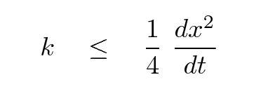
Using even smaller fractions in this condition may be beneficial, up to a point -- when the fraction is (1/6), truncation errors tend to be minimized.
Note that these conditions hold only for the algorithm we've examined: a simple, Euler-like method which uses the current second derivative in position to compute the current first derivative in time, and assumes that the first derivative is constant over the entire timestep. There are more complex algorithms which are less likely to become unstable, which means that one might use larger time-steps and/or position-steps to reach the goal more quickly.