You've seen it in one dimension: heat flows through a long, thin rod. Today, we look at the very similar situation in two dimensions: heat flows through a flat plate.
Once again, we will assume that the flow of heat is steady, and so we'll deal only with the equilibrium temperature of the plate. We will also adopt similar boundary conditions: instead of specifying the temperature at each end of the rod, we'll specify the temperature along the four edges of the plate.
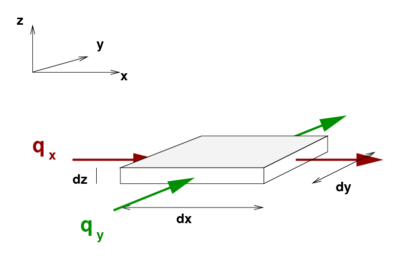
Here's the basic picture: the plate runs in the X and Y directions, but is very thin in Z. The figure below shows one small element of the plate, with width dx and dy and thickness dz.
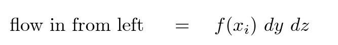
We assume that no heat enters or leaves the plate through the upper and lower faces; in other words, there is no flow of heat in the Z-direction. However, heat does flow in the X- and Y-directions, as shown by the brown and green arrows, respectively. We can describe the amount of heat flowing into this little section through the left edge as
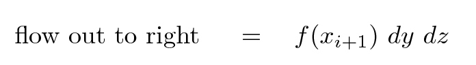
and the heat flowing out through the right edge as
If we demand that the flow into and out of the section is equal in the X-direction, we can derive
But we can go through exactly the same analysis in the Y-direction to derive
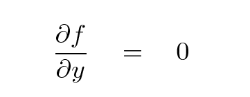
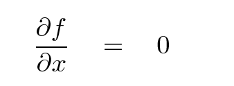
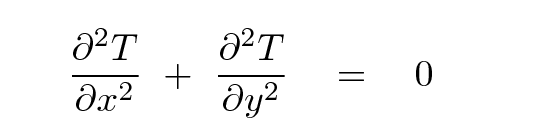
If we describe the plate by a temperature T(x,y) instead of by the heat flowing through it, then we can determine that
Consider one element of a 2-D array representing temperature.
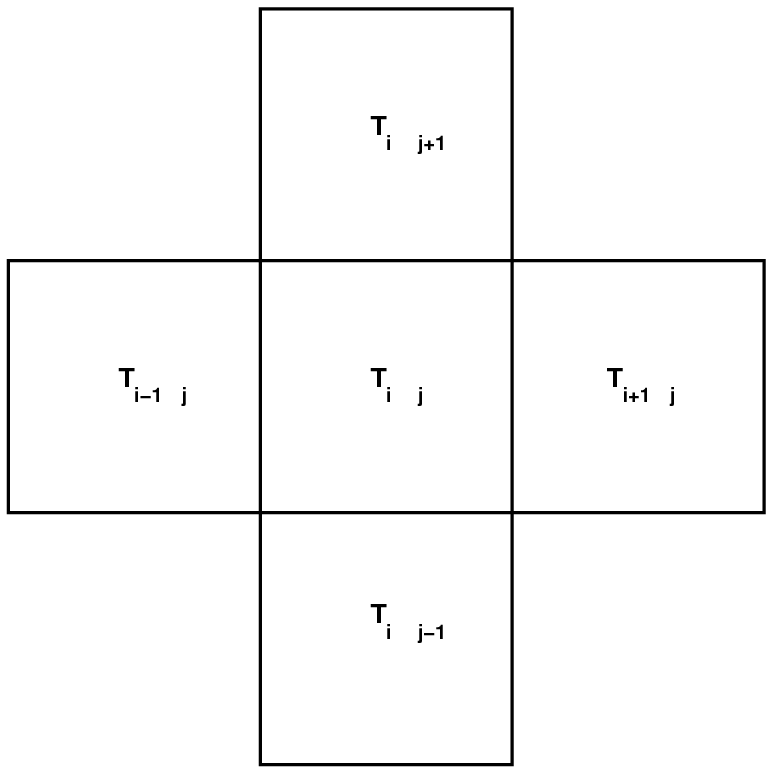
  Q:  What is a difference equation for the flow of
          heat in the X-direction through this element?


  Q:  What is a difference equation for the flow of
          heat in the Y-direction through this element?


  Q:  Write this as a system of 2 equations --
          how many unknowns are there?


  Q:  Write this as a system of 1 equation --
          how many unknowns are there?
Uh-oh. How can you deal with THIS system of equations? Well, we get some help from the boundary conditions, of course.
One way to approach the problem is iteratively. We can re-write the equations above like so:
                 T      +  T      +  T      +  T
                  i+1,j     i-1,j     i,j+1     i,j-1
    T     =     --------------------------------------
     i,j                         4
In other words, the temperature of the central section is the average of the temperatures of the surrounding sections.
So, if you simply guess some initial temperatures for each grid point, you can use the equation above to compute new, improved temperatures, then repeat as needed until the solution converges.
One way to improve the performance of an algorithm of this sort is to use a weighting factor when determining the temperature for the next round:
If you set λ = 1, then the solution may converge quickly ... or it may go crazy. If you set λ to a relatively small value, the solution may converge more slowly ... but it may be more stable.
Just as we did with the thin rod, we can use an approach based on linear algebra. It will be a bit more involved this time, though: if we look at a plate with N-by-N elements, then we'll be solving a set of equations with
Can it be done? Sure. Can you at least start the process? You might consider for practice a simple little 3x3 plate ....
If you choose to attack this problem using linear algebra, rather than an iterative approach, you will find that it can be reduced to a matrix equation that looks like
A * x = b
where A is an N2-by-N2 matrix, x is a vector of length N2 of unknown temperatures, and b is a vector of length N2 containing combinations of the temperatures along the edges of the plate.
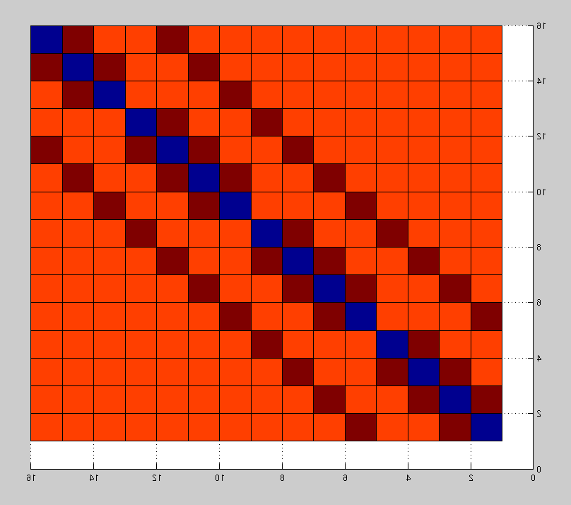
If you look carefully, you'll find that the matrix A is rather "sparse." Here's what it looks like for the case of N = 4.
    -4     1     0     0     1     0     0     0     0     0     0     0     0     0     0     0
     1    -4     1     0     0     1     0     0     0     0     0     0     0     0     0     0
     0     1    -4     1     0     0     1     0     0     0     0     0     0     0     0     0
     0     0     1    -4     0     0     0     1     0     0     0     0     0     0     0     0
     1     0     0     0    -4     1     0     0     1     0     0     0     0     0     0     0
     0     1     0     0     1    -4     1     0     0     1     0     0     0     0     0     0
     0     0     1     0     0     1    -4     1     0     0     1     0     0     0     0     0
     0     0     0     1     0     0     1    -4     0     0     0     1     0     0     0     0
     0     0     0     0     1     0     0     0    -4     1     0     0     1     0     0     0
     0     0     0     0     0     1     0     0     1    -4     1     0     0     1     0     0
     0     0     0     0     0     0     1     0     0     1    -4     1     0     0     1     0
     0     0     0     0     0     0     0     1     0     0     1    -4     0     0     0     1
     0     0     0     0     0     0     0     0     1     0     0     0    -4     1     0     0
     0     0     0     0     0     0     0     0     0     1     0     0     1    -4     1     0
     0     0     0     0     0     0     0     0     0     0     1     0     0     1    -4     1
     0     0     0     0     0     0     0     0     0     0     0     1     0     0     1    -4
It's not quite diagonal, but it's not far from it, either. You can see that more clearly, perhaps, if we make a surface plot showing values of this matrix.
N = 4
N = 10
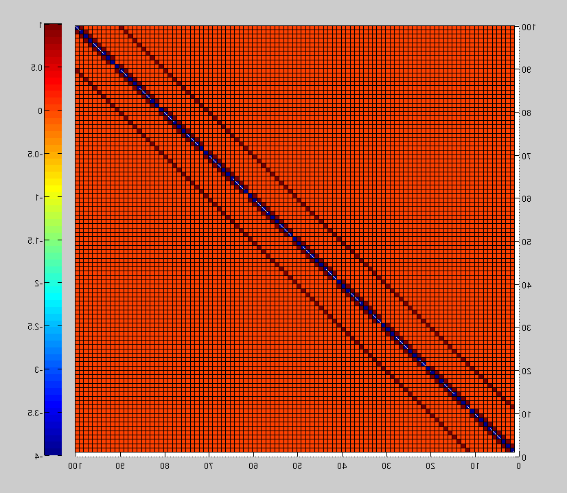
You may find that, when a matrix is relatively sparse, there could be some ways of solving the equation which run more quickly than others ....
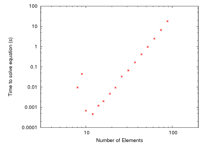
Note that the time rises very rapidly with N: