 Copyright © Michael Richmond.
This work is licensed under a Creative Commons License.
Copyright © Michael Richmond.
This work is licensed under a Creative Commons License.
We have data: measurements of voltage as a function of time from a big black box. The box creates spikes of voltage which are FIXED to have a gaussian shape, with an amplitude of 1 volt, and a FWHM of 1 second. The only question is: when does each spike occur?
Here's an example of one spike:

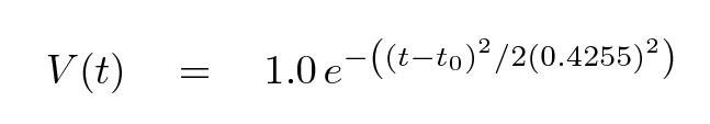
And here's the mathematical model we are going to fit to the data:
In this ideal case, in which the data is noiseless and we have a model with just one free parameter, it's not too hard. We can define a metric which measures quantitatively the goodness of fit:

Then, we can generate data for a range of possible t0 values, and compute the metric for each of our guesses. For example, if we choose
t0 = 1.0, 2.0, 3.0, 4.0, ....
then we'll find these values of our metric K2:

  Q:  What is the "best" value for the time of the spike?


  Q:  Is that really the best we can do?  What should
      we do as our next step?
Right. Now that we know that the best time lies somewhere around t = 12, we can make another set of models, this time choosing times close to 12 seconds.
t0 = 11.0, 11.1, 11.2, 11.3, 11.4, ....
When we compare this finely spaced set of models to the data, we'll find new values of our metric K2:

  Q:  What is the "best" value for the time of the spike?


  Q:  Is that really the best we can do?  What should
      we do as our next step?
Okay, okay. You get the idea. When there is just one free parameter, and the measurements are so clean, and the model is so simple ... it's easy: just focus in on a smaller and smaller region of the parameter, and there you go.
In real life, measurements often are contaminated by noise, from many different sources. In some cases, it is reasonable to conclude that the noise has a gaussian distribution. Consider, for example, voltage measurements in the presence of random gaussian noise with a standard deviation of σ = 0.1 volts.
What happens if we follow the same procedure and try to fit a model to this data?

Hey! That's not so bad.
  Q:  Why is the fit metric so "smooth" compared
      to the measurements?
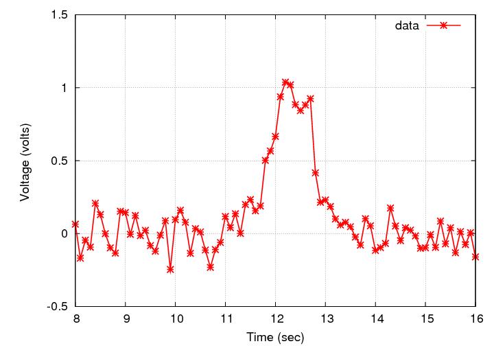
But what if the noise is larger? In the case below, the noise per measurement is about 1/3 of the maximum signal.

When we run our fitting procedure, we still get a smooth-looking result ... but is it correct?

It surely would be nice to have some idea for the uncertainty in the value of the fitted parameter, wouldn't it?
  Q:  How can we estimate the uncertainty
      in this time we've just determined?
There are several methods scientists use to estimate the uncertainties in the values of fitted parameters. I will mention here one that is relatively simple to understand, and, with the aid of the computer, relatively simple to perform. Although it may take some time to calculate, the idea here is fundamental; we can extend it to situations in which there are multiple parameters, too.
For example, I looked at this set of measurements:
Using the measurements which seemed far from the peak, I computed a mean value of 0 volts, with a standard deviation of 0.3 volts. So, my next step was to generate an artificial signal in a gaussian shape, with an amplitude of 1.0 volts and a FWHM of 1.0 seconds, centered on some particular value: I chose 12.89 seconds. Next, I entered a big loop:
Here are the first few results. Note that I used a grid of 0.1 seconds when I was computing models in my K2 fitting procedure.
t = 12.8, 12.9, 12.9, 12.9, 12.9, 12.8, 13.0, 12.9, 12.8 .....
When the noise in the original data had a stdev of about 0.3 volts, I found that the scatter in my fitted times was about 0.08 seconds.
Ta-da! I wanted some estimate for the precision of my K2 fitting procedure, and now I have one.
One of the things I learned is that it's probably worthwhile for me to run my fitting procedure using more finely spaced times.
Copyright © Michael Richmond.
This work is licensed under a Creative Commons License.