Using higher-order methods, in simple situations

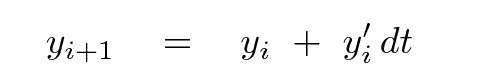
Euler's method is a common choice to solve a differential equation numerically. Why? Because it's easy to understand and easy to implement in any language, and, in many cases, it works well enough. Occasionally, however, the inaccuracy of this approach is just too large -- the results end up too far from the correct values. What then?

Well, if the situation is "simple", one can apply a more accurate method which uses the same basic approach as the Euler method. What does "simple" mean in this context? It means the derivative of the function of interest does not depend on the value of the function itself.

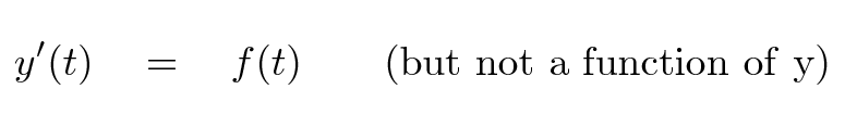
For example, let y be the height of a ball falling in a vacuum near the Earth's surface. The derivative of y(t) is simply

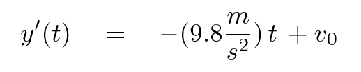
Suppose we start with initial conditions y(t = 0) = 100 m and y'(t = 0) = 0 m/s. Use Euler's method to fill in the table below.


  t              y'            y  
 (s)           (m/s)          (m)
-----------------------------------------------
  0              0            100

  1          

  2   

  3   

-----------------------------------------------

Are all these values exactly correct? If not, why not?

A graphical look at the problem

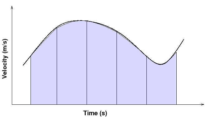
One way to think of integration is the process of finding the area under the curve; in this example, we are using the area under the curve of velocity versus time to find displacement. Euler's method is equivalent to breaking this region into a series of rectangles. The height of each rectangle is the value of the velocity at the start of each timestep. If the velocity changes during a timestep, then the method doesn't do a very good job of computing the area under that section of the curve.

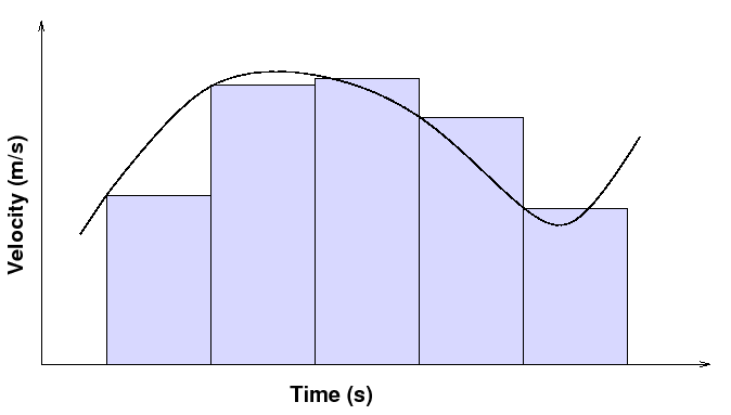
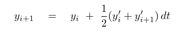
It's clearly a better idea to take into account the change in the value of the derivative over a single timestep. For example, we could evaluate the velocity at the beginning of a timestep, and again at the end of the timestep, and draw a trapezoid to include these two velocities. The area under each trapezoid is a better match to the area under the continuous curve.

We can put this idea into an algorithm like so:

Try using this approach to solve the falling ball again.


  t              y'            y  
 (s)           (m/s)          (m)
-----------------------------------------------
  0              0            100

  1          

  2   

  3   

-----------------------------------------------

Going to higher orders

As long as we can compute the derivative of the function of interest -- in this case, the velocity of the ball -- at arbitrary times, we can achieve more and more accurate results by adding more and more values of the velocity within each timestep. You may have heard of Simpson's method, which evaluates the velocity at the start, middle, and end of each timestep, then combines them with a particular choice of weights.

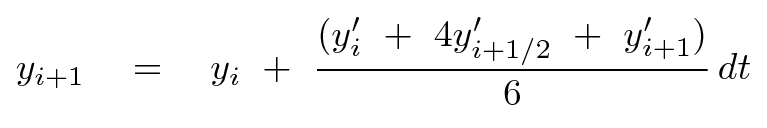
In graphical terms, this is equivalent to using three measurements to fit a parabola to the function within each timestep.

The accuracy of increases with the the number of times one evaluates the derivative within each timestep. That's the good news. The bad news is that it takes a computer time to calculate these derivatives, and so slows down the execution of the program.

Advantages of going to higher orders:

error in each step decreases
can use larger steps and still improve accuracy

Disadvantages of going to higher orders:

increased time to perform each step
increased complexity of code: more chances for errors to creep into the software, harder to find and remove them