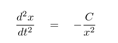
We are going to shift gears now and move from one sort of physical situation to a different one. For the past four weeks, we've been looking at the motion of objects under the influence of gravitational forces. The basic differential equation we've been solving looks like this:
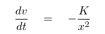
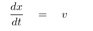
Our approach has been to break that second-order equation into a pair of first-order equations:
There are a number of techniques to deal with this set of first-order equations, and you've had a chance to see the circumstances which might favor one or another.
But we will turn now to a very different physical situation: instead of following the motion of ideal compact objects through space, we will now be studying the flow of heat through a solid material. As you might imagine, this will lead to a very different sort of differential equation, which will in turn require some new approaches in our solutions.
We can gain some understanding of the way that heat flows by starting with a very simple analogy: the flow of water through a long, thin pipe. Imagine a pipe which flows from west to east:
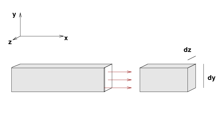
Let's set up a coordinate system in which the X-axis runs from west to east, the Y-axis vertically upward, and the Z-axis north to south (out of the figure above). We can define the quantity
   f(x)    =     the rate at which water flows
                 through the pipe at location x
                    (kg per sq. meter per second)
Let's zoom in on one little section of the pipe, at location xi. so the cross-section area is dy dz. To the left and right of this section are its neighboring sections, xi-1 to the left, and xi+1 to the right.
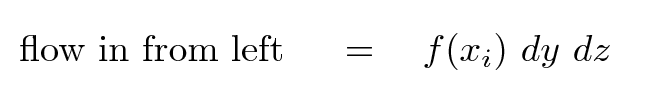
The cross section of the pipe is square, with length dy and dz. So, the rate at which water flows into this section from the left is
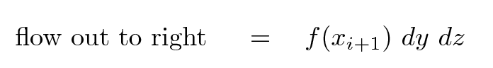
The rate at which water flows out of the pipe into the section to its right is
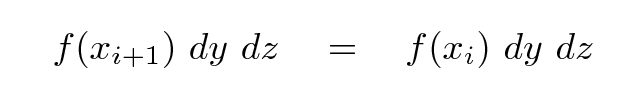
So, if water is flowing through the pipe in a steady state -- in a manner which doesn't change with time -- then the amount flowing in from the left must equal the amount flowing out to the right. In other words,
If we define the small distance between adjacent sections of pipe as
then we can write this condition for steady-state flow of water as
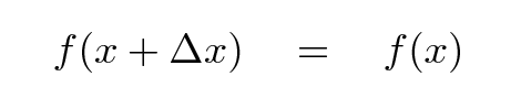
In other words, in a steady state, the flow of water into each section of the pipe is equal to the flow out of that section.
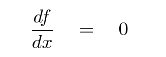
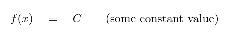
The solution to this differential equation is simple: the flow rate f(x) must not change with position, so
Let's return to the real topic of our work, the flow of heat through a solid. If we define the quantity q(x) to represent the flow of heat through a long, thin rod at location x, and we demand that the solution be independent of time (i.e., in the steady state), we can derive a very similar sort of relationship.
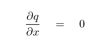
Note the change in notation: since we are (soon) going to be dealing with multiple spatial dimensions, and the flow of heat may vary differently in each direction, we must use partial derivatives. In our previous work on the motion of objects due to gravity, we took derivatives with respect to a single quantity -- time -- and so never needed to use partial differentiation.
Now, the reason things are about to get a bit more complicated is because we don't usually describe a physical system in terms of q(x) -- we don't often list the flow of heat at all points in a material. It is more common to describe the TEMPERATURE of a material, T(x). Temperature is related to the the flow of heat, of course, and one can define that relationship in the following manner (as a certain Mr. Fourier did)
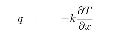
where k is called the coefficient of thermal conductivity, and varies from material to material.
Q: Why is there a negative sign in this equation?
Okay, we have one differential equation for q(x) as a function of position, and a second equation for T(x) as a function of q(x), so we can put those two together and derive an equation for the temperature as a function of position.
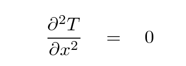
This is a one-dimensional version of what is sometimes called Laplace's equation. There are other versions in two- and three-dimensional situations, and we'll deal with those later on. For now, however, let's stick with the one-dimensional case.
One of the conditions we used in deriving the Laplace equation for the long, thin rod was that the flow of heat into one little section of the rod should be equal to the flow of heat out of that same section. If we go back to the water analogy for a moment, the amount of water flowing into a little section of pipe should equal the amount flowing out. That's just common sense; after all, if more water flows in than flows out, there will be a build-up of water in that one little section of the pipe, which certainly can't go on forever in the steady state.
Well, it can't go on forever -- unless that section of pipe has a leak. If one considers the flow of water through a pipe, one can imagine several ways that the flow in and out of one section through the left and right walls might not be equal.
We use the terms sources and sinks of water to describe these extra factors which affect the flow of water through our pipe.
In the same way, there can be sources and sinks of heat along a long, thin rod. A chemical reaction at location x = 5 m might produce extra heat at this spot; or a copper wire attached at x = -20 m might carry heat away to an external radiator. We can account for any sources or sinks of heat by modifying the differential equation so that it reads
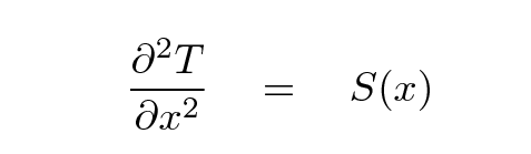
where S(x) describes the sources and sinks. When the right-hand side is not zero, we call this equation Poisson's equation instead of Laplace's.
If you are given a heat conduction problem, make sure that you have the proper boundary conditions. Without them, there may be no solution.
Here's a really simple problem: a rod is attached to heaters on both ends. The left-hand end is kept at 100 K, the right-hand end at 50 K. Treat the rod numerically as N = 2 small sections.
      index  i                  1         2

      Temp  Ti         100      T1       T2       50
What are the steady-state temperatures of the two sections? Well, if we approximate the second derivative using numerical differences, we get for the first chunk i=1
( T2 - T1 ) - ( T1 - 100 ) = 0
Hmmm. One equation, two unknown temperatures. Can't be solved.
For the second chunk, we find
( 50 - T2 ) - ( T2 - T1 ) = 0
Again, one equation, two unknown temperatures.
But if we put these N = 2 equations together, we end up with 2 equations for 2 unknowns. Now THAT is a system of linear equations which we can solve for the unknown temperatures.
  Q:  What are the temperatures T1 and T2
      which solve the system of equations?
There's (at least) one more way to work on this sort of problem, which involves using a starting guess and then working iteratively to improve it.
Consider the same problem: a rod is attached to heaters on both ends. The left-hand end is kept at 100 K, the right-hand end at 50 K. Treat the rod numerically as N = 2 small sections.
      index  i                  1         2

      Temp  Ti         100      T1       T2       50
We don't know what the temperatures T1 and T2 are ... but we do know that in the steady state, we should have
( T2 - T1 ) - ( T1 - 100 ) = 0
We can do a little algebra to solve for T1 in terms of the other quantities.
           T2  +  100  -  2 T1   =   0

   so

           T1   =   (1/2) ( T2 + 100 )
In a similar way, we can derive that
T2 = (1/2) ( T1 + 50 )
Let's start by guessing that both temperatures are T1 = T2 = 0. If that's so, then the second derivative at the position of the first chunk becomes
        ( T2  -  T1 )   -   ( T1 - 100 )   =   0

         ( 0  -  0 )    -   ( 0  - 100 )   =   100
Whoops! This is supposed to yield zero, but it certainly does not. If we check the second derivative at the location of the second chunk, we find another failure:
        ( 50  -  T2 )   -   ( T2 - T1  )   =   0

        ( 50  -  0  )   -   ( 0  -  0  )   =   50
So, our initial guess didn't work. Rats. But we can use the initial guess to find a better value. For T1, for example,
      new  T1   =   (1/2) ( T2 + 100 )

                =   (1/2) (  0 + 100 )

                =    50
  Q:  What is the new predicted value for T2?


  Q:  Use these new values to compute the second
      derivatives at the location of each chunk.
      Do the derivatives equal zero now?


  Q:  What are the values of T1 and T2 after
      a third iteration?