 Copyright © Michael Richmond.
This work is licensed under a Creative Commons License.
Copyright © Michael Richmond.
This work is licensed under a Creative Commons License.
A big black box provides measurements of voltage. We find that most of the measurements are zero. Occasionally, however, the voltage increases for a short period, then decreases again, like this:

Let's choose to compare these measurements to a simple model: a gaussian function like this:
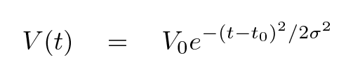
Moreover, after a bit of experimentation, we find out that the width of these pulses is very regular: the FWHM (Full Width at Half-Maximum) is always 1.0 seconds, which means that the parameter σ in the equation above is

That leaves us with exactly 2 free parameters: the peak amplitude V0, and the time of the peak t0. How can we find the combination of these two parameters, so that our model best matches the observations?
As a metric, we'll choose the sum-of-squares-of-differences quantity (which is similar to the chi-squared statistic):
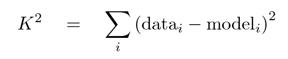
Our job: find the values of V0 and t0 which minimize K2.
One approach is very simple: we can create a 2-D grid which covers some range of values of amplitude V0, and some range of values of time t0. We can compute the K2 metric for all locations on the grid, and then choose the location which yields the smallest value. We might iterate several times to "zoom in" on the location.
Pseudocode for this procedure might look like this:
% select a starting point
guess_amp = 4.0;
guess_t = 7.0;

% select a range around the starting point
amp_range = 1.0;
t_range = 0.5;

% break each range into this many pieces
n = 100;

% iterate 5 times, zooming in on the best location
for i = 1 : 5

  % loop over all possible amplitudes
  for amp = min_amp to max_amp

     % loop over all possible times
     for time = min_time to max_time

         % compute the k-squared metric using this amp, time
         k_squared = compute_ksquared

         % is this value smaller than the best one found so far?
         if (k_squared < min_ksquared)
            min_ksquared = k_squared
            best_amp = amp
            best_time = time
         end

     end

  end

  % now recenter the range of amplitudes and times on best values
  %    and decrease the range of each

end
Will this work? Yes, probably. But it might take quite a while.
  Q:  How many times will we have to compute the K-squared
      metric in this particular example?
When there is just a single parameter to fit, this is often the best way to go: it's easy to write the code, and easy to understand. But if there are 3, or 5, or 10 free parameters, the time it takes to cover a reasonable range in each parameter with a fine grid can become much too long.
A different approach can save a lot of time. Instead of trying to find the very best spot by an exhaustive search -- which wastes lots of time looking in the wrong places -- let's make a quick scan of the region around some initial guess, figure out which way will lead us to the goal, and then head in that direction.
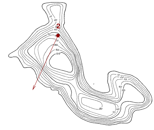
It may help to consider an analogy. Suppose we want to reach the very peak of a mountain which has a complicated shape. We start somewhere far from the peak.
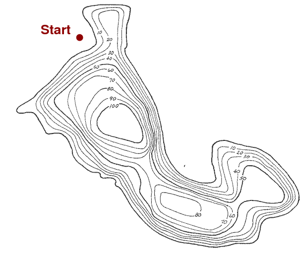
Our method is simple: look for the direction which goes uphill most directly from our current location, and start walking in that direction.
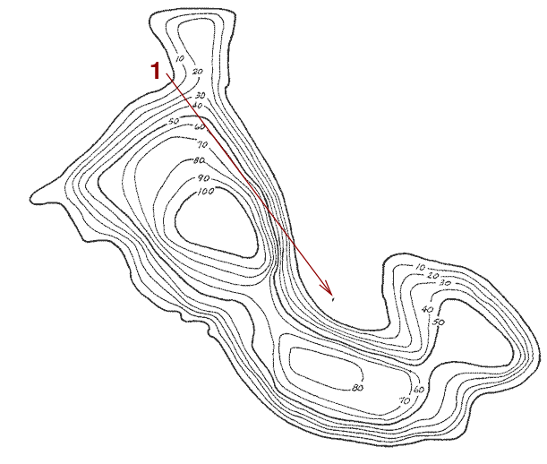
Keep walking as long we continue to go uphill. But if we reach a point at which moving further ahead would take us DOWNhill, then stop.

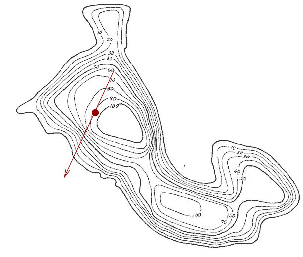
Now, while standing here, once again scan the local landscape and identify the direction which goes uphill most directly.
Walk along this path until the path begins to head downhill, then stop.
Once more, scan the local landscape and find the uphill direction.
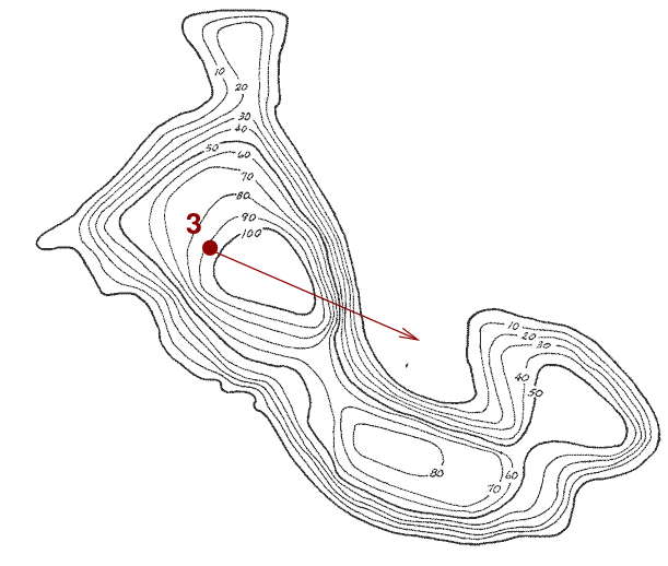
Walk forward, checking as always that we are still going uphill. When moving forward would cause us to go downhill, stop.
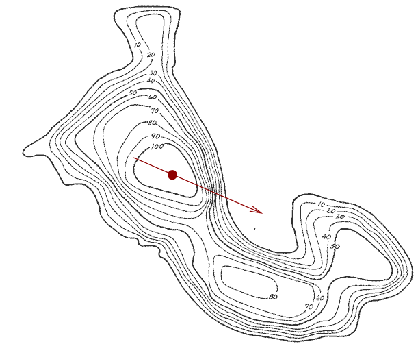
And, voila!, we have made it to the top of the hill.
This procedure is known as the method of steepest ascent. Make sense, doesn't it?
Now, first of all, in our problem, we are seeking a minimum in the value of K2, not a maximum, but that's easy to fix: just modify the procedure so that we scan the landscape and look for the direction which takes us DOWNhill most rapidly.
The real question here is -- how can we identify the "direction" to move? What does that even mean?
Let's define a function f(A, t) which takes two parameters -- a guess at the amplitude of the voltage spike and the time of its peak -- and uses them to compute some number (yes, this should look familiar).
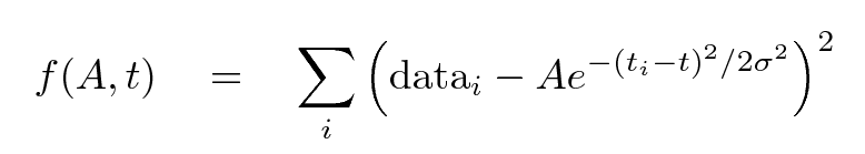
If we take the derivative of f with respect to A, we'll find a measure of how quickly f is changing with respect to A; a positive value means that if we increase A, we also increase f. Likewise, if we take the derivative of f with respect to t, then we'll find out how quickly, and in which direction, the function f changes with respect to changes in t. The gradient of the function is simply a vector formed by these partial derivatives.

On a 2-D map (or a 3-D map, or a 9-D map), the gradient points toward the steepest local "uphill" direction.
If we want to go "downhill", we can just compute the gradient, then go in the opposite direction.
But -- wait! Our function f looks pretty complicated. How can we take the derivative with respect to the parameters?
Well, even if the function is complicated, we can still find an approximate derivative numerically. Suppose we have some starting values A1 and t1. We can compute a numerical derivative of the function with respect to each variable by adding and subtracting just a little bit to each parameter and computing the change in the function.

For example, let's go back to the example of the voltage coming out of a big black box. One set of measurements yields a single spike:
We begin with a guess that the spike has an amplitude of 4 volts and is centered at 7 seconds. At this starting point, we can compute K2: it has a value of 99. Surely we can find a pair of parameters which yields a smaller result.
If we calculate the K2 statistic in this general area, we can see that we aren't too far from the minimum value. In the graph below, amplitude is on the horizontal axis and time on the vertical axis.
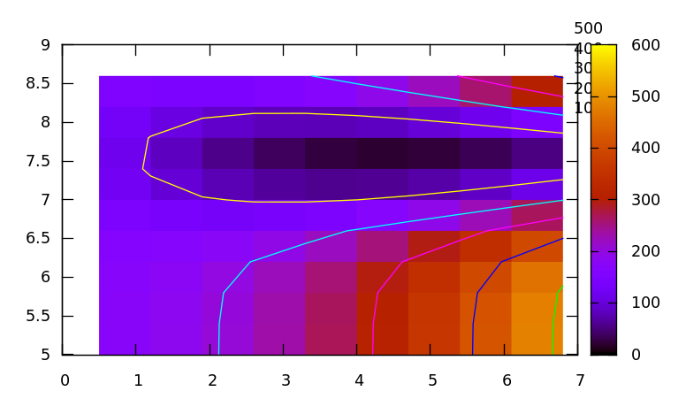
In order to use the method of steepest descent (remember, we want to go DOWNHILL in order to find the miminum value of the statistic), we must first compute the gradient at our initial location of (4 volts, 7 seconds). In order to compute the numerical derivative with respect to amplitude, let's add and subtract 0.5 volts. I'll do some of the math for you.
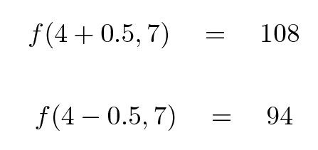
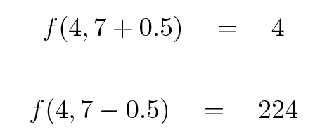
  Q:  What is the gradient of f at our starting point?


  Q:  Which direction should we move to go downhill most rapidly?
Okay, it's clear that we should move toward SMALLER values of amplitude, and LARGER values of time. We can also tell that changes in time are more important than changes in amplitude -- by about a factor of 10 or so. So, when we move, we want to move mostly in time, with just a relatively small change in amplitude. How can we do that?
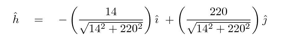
One way to proceed is to create a vector which points in the right direction. If we define the gradient as
then we can compute a unit vector in its direction like so:
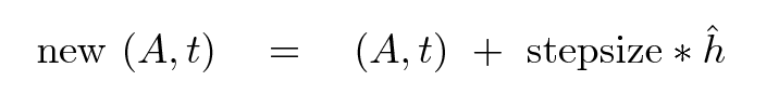
Now, if we want to move "forward", toward the local downhill direction, we can simply pick some stepsize and compute a new value of the parameters like this:
stepsize     amp       time       K2
-------------------------------------------
 0.0000    4.0000     7.0000    99.8941
 0.1000    3.9941     7.0941    73.8937
 0.2000    3.9881     7.1881    50.1717
 0.3000    3.9822     7.2822    30.1702
 0.4000    3.9763     7.3763    15.1884
 0.5000    3.9704     7.4704     6.2411
 0.6000    3.9644     7.5644     3.9424
 0.7000    3.9585     7.6585     8.4330
 0.8000    3.9526     7.7526    19.3635
 0.9000    3.9467     7.8467    35.9358
 1.0000    3.9407     7.9407    56.9969

-------------------------------------------
Aha! This table indicates that eventually, moving in this direction stops going "downhill" and starts moving "uphill", toward larger values of K2, and thus toward fits which are less good. That means that we should stop when we reach A = 3.96 volts and t = 7.56 seconds. We should then once again compute the local gradient, pick a new direction of steepest descent, and walk in THAT direction until we reach another minimum.
We can follow this procedure several times, moving closer and closer to the minimum value of K2 and so closer and closer to the "best" values of amplitude and time.
Let's try this method on our example.
 iter     amp       time          K2
------------------------------------------
  0      4.0000    7.0000       99.8941
  1      3.9644    7.5644        3.9424
  2      4.0221    7.5221        3.5686
  3      4.0416    7.5527        3.0769
  4      4.3230    7.5091        1.6658
  5      4.3318    7.5503        0.9144
  6      4.6626    7.5404        0.0444
  7      4.6629    7.5494        0.0024
  8      4.6635    7.5503        0.0021
  9      4.6644    7.5496        0.0019
------------------------------------------
That's pretty impressive.
The important thing is that we didn't have to go through the long, time-consuming calculation of K2 very frequently. In this example, I called a function to compute K2 only 191 times. That may sound like a lot, but if I had tried the brute force method, it would have taken a LOT more time.
  Consider using the brute force method,
  with a square grid ranging from

          (3, 6)    to    (5, 8)


  Q:  In order to keep the number of calculations
      of K2 under 200, what is the largest
      grid one could use?


  Q:  What would be the precision of a "best guess"
      at (amp, time) if you used that grid?


  Q:  Suppose you wanted to match the precision
      of this method of steepest descent;
      it found both amplitude and time to a
      precision of about 0.001 volts and 0.001 seconds.

      How large a grid would you need?

      How many evaluations of K2 would that require?

      How much longer would that take to compute?
Copyright © Michael Richmond.
This work is licensed under a Creative Commons License.