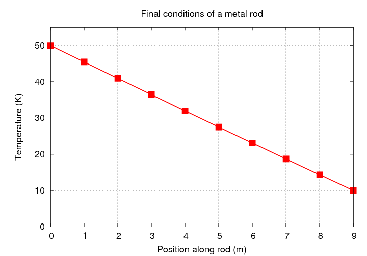
So far, we've restricted ourself to steady-state solutions: given a metal rod with the temperatures fixed at each end, what is the equilibrium temperature as a function of position? The answer is pretty simple:
But what if we wanted to start the rod at some non-equilibrium condition -- like this,
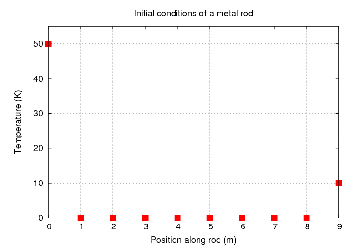
and then watch to see how long it would take the temperature to reach that equilibrium state. Perhaps it might be interesting to watch the temperature evolve, as heat "leaks" into the rod from both ends.
In order to follow the changing temperature as a function of time, we need some physics.
We need to know two separate (but related) things:
Let's look at one small section of a metal rod. The section has a width dx. We are interested in the amount of heat flowing through this little section of the rod. We'll use the convention that the rate at which energy flows through the section, q(x), is positive if the energy flows in the positive X direction.

How large is the rate of heat flow through this section? Mr. Fourier found that one can write down the magntiude of the heat flow in terms of several material properties:
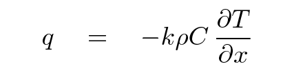
where
    q             is rate of energy flowing through section
                           (J / m^2*s)

    k             is the thermal diffusivity of material
                           (m^2 / s)

    ρ             is the density of the material
                           (kg / m^3)

    C             is the heat capacity of the material
                           (J / kg*degC)

    T             is the temperature of the material
                           (degC)

    x             is position
                           (m)
Note the negative sign: if the temperature increases to the right, then the flow of heat will go to the LEFT.
Now, suppose we do know the amount of heat flowing INTO the section from the left end, and flowing OUT OF the section from the right end. How does the temperature of the section change as a result?
Well, if the amount of heat flowing INTO the rod exactly balances the heat flowing OUT OF the rod, the amount of thermal energy inside the rod will be constant -- and so will its temperature. The only way to change the temperature is to make the heat flow larger at one end than the other. If we do that, then the difference in those flow rates, multiplied by time, is the amount of energy going into the section; and that extra energy will cause the temperature to change.
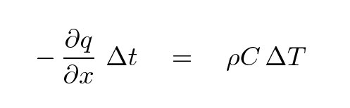
where
    q             is rate of energy flowing through section
                           (J / m^2*s)

    x             is position
                           (m)

    Δt            is the time over which the heat flows
                           (s)

    ρ             is the density of the material
                           (kg / m^3)

    C             is the heat capacity of the material
                           (J / kg*degC)

    ΔT            is the change in the temperature
                           (degC)
Again, note the negative sign: if the gradient of heat flow is positive, so that q(x + dx) is greater than q(x), then energy flows OUT of the section; in that case, its temperature must decrease, so ΔT must be negative.
So, now we have one equation for q, and another one for the derivative of q with respect to x.
  Q:  Take the derivative of the first equation
      with respect to position x.


  Q:  Set the resulting equation equal to the
      second equation.


  Q:  Derive an expression for the change in
      temperature of the section over time.
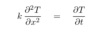
Great! If we have a map of the temperature of a metal rod at some particular time, and we know the diffusivity of the material, then we can figure out how much the temperature of each little piece of the rod will change over some little timestep. In other words, we can follow the evolution of the temperature of a rod with time.
Given arrays of temperature Ti and position xi for a bunch of little sections i = 1, 2, 3, ..., N, the thermal diffusivity k, and a timestep dt, we can compute a numerical second derivative and use it to estimate the new temperature at each position.

Warning, warning, danger Will Robinson!
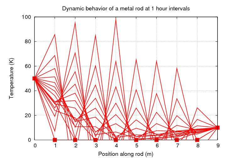
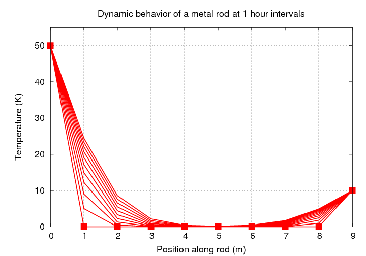
This looks simple enough, but, as we will see, this is an example of a situation in which numerical instability can easily arise. If we don't choose our timestep (and space-step) carefully, our "solution" will look less like this:
and more like this: