 Copyright © Michael Richmond.
This work is licensed under a Creative Commons License.
Signal Versus Noise (some theory)
There are a number of factors which affect the quality of
photometry of star in a CCD image.
One is the exposure time: the longer the exposure time,
the higher the signal in a star, and so the more precise
the measurements.
Of course, if one exposures too long, one will saturate the
CCD, which ruins the measurements.
But how long an exposure time is necessary?
The answer depends on your goal.
If you simply want to verify that
an object is present at a particular location,
you may accept a very faint, barely noticeable dot of light.
If you want to measure the position of
an asteroid to an arcsecond, you would need
a little more signal.
If you want to make a very rough estimate
of magnitude, to ten percent, say, then
you might need more signal.
And if the goal is to look for tiny variations
in light of a variable star, you might need
to expose long enough that the star comes
close to the non-linear regime.
So how can you figure out the appropriate exposure
time for a given project?
There are two approaches:
- Consider this exchange from Calvin and Hobbes:

You can do exactly the same thing with your astronomical observing:
take a series of images with increasing exposure times, and
measure the object of interest on each one.
The shortest exposure which provides enough precision for your
goal is the right length.
This actually isn't a bad idea if you have huge amounts of
observing time. On the other hand, if you are given just a single
night on a big telescope, you probably won't want to waste any
time taking a series of pictures, most of which turn out to be
useless.
- Calculate the signal from your object for a set of
exposure times. There will be a number of different
sources of noise in the image -- determine the amount
of noise from each and add them up.
The ratio of signal-to-noise (S/N) yields the uncertainty
in the measurement of stellar brightness:
                                     1
      fractional  uncertainty  =   -----
                                    S/N
So, for example, if the S/N ratio is 50, the photometry will
have an uncertainty of 0.02, which is the same as 2 percent,
and which is approximately 0.02 magnitudes.
An extended analogy on the statistics of counting
Your job is to figure out the appropriate
cash reserves for McKing restaurants --
the amount of money which should be kept in the
registers.
You decide it is important to know the answer to the question
How many customers each hour pay with a $20 bill?
So, you do a little research.
You go to a local store in Henrietta
and count the number of customers who
need change for a $20.
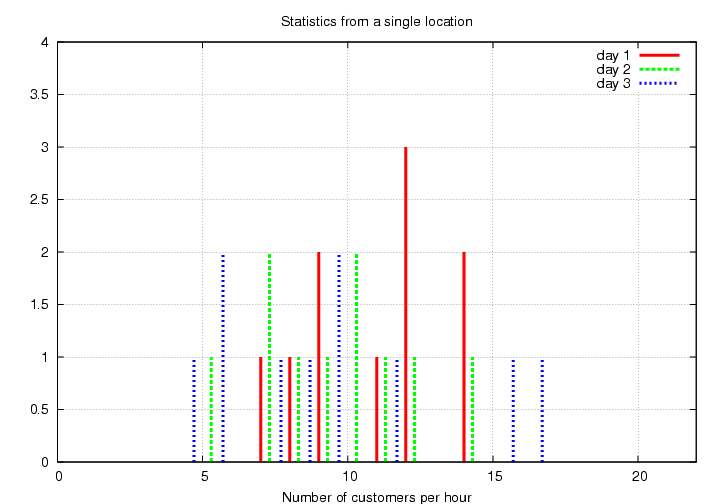
You find
      Hour-by-hour counts throughout the day

  Day 1:  11    12     9    12     9     7    14    14    12     8
  Day 2:   7    10    12     5     9    14    10    11     8     7
  Day 3:  10     5     9     6    17    10    12     6    16     8
A more convenient way of displaying
this information is in the form of a
histogram.

There seems to be quite a bit of variation from
day to day.
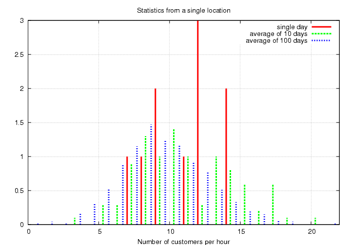
So you extend your period of study over 10 days,
then 100 days, and take the average numbers
during each period.

Hmmm.
The distribution becomes smoother and more symmetric
with more time, doesn't it?
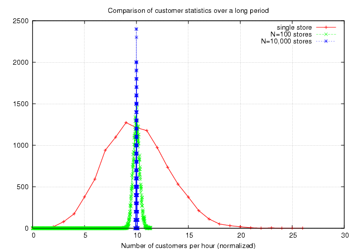
If you were to watch the same store for 3 years,
you might get a distribution like this:

Exercise:
- What is the mean value of this distribution?
The standard deviation is (I measured it myself)
about 3.1 customers per hour.
That is, the scatter around the mean value
is about +/- 3 customers.
- What fraction of the mean value is the scatter?
That is, by what percent of the average
number of customers per hour does the
measurement fluctuate?
Now, you want to get a better idea for this
value, because it turns out to be crucial for
figuring out how much cash you need to keep
in the store.
So, instead of looking at a single
store, you decide to hire people to make
similar counts at all the restaurants in
Monroe County.
There are N = 100 restaurants,
so you will find a much larger number of
customers per hour -- at all stores --
who pay with $20 bills.
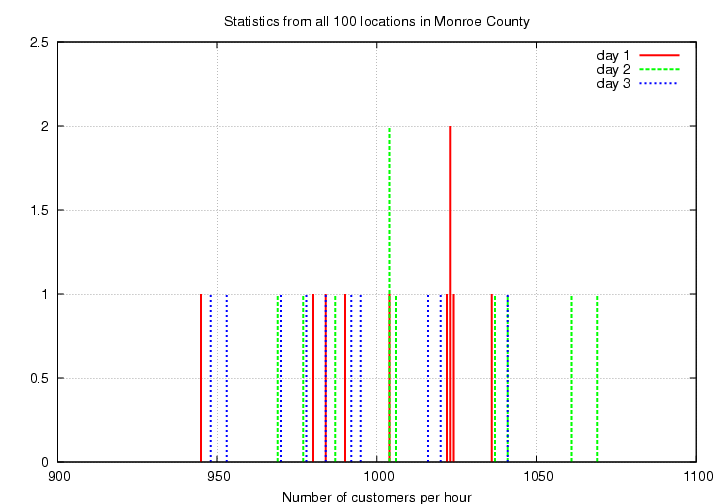
Here are the raw counts for the first few
days of your big study.
      Hour-by-hour counts throughout the day

  Day 1:  1023   945  1004   984  1024   990  1023  1036   980  1022
  Day 2:  1061  1041  1004  1006   977  1037  1069  1004   987   969
  Day 3:   953   992   970  1041  1020  1016   984   978   948   995
Again, you decide to use a histogram to display
this information.

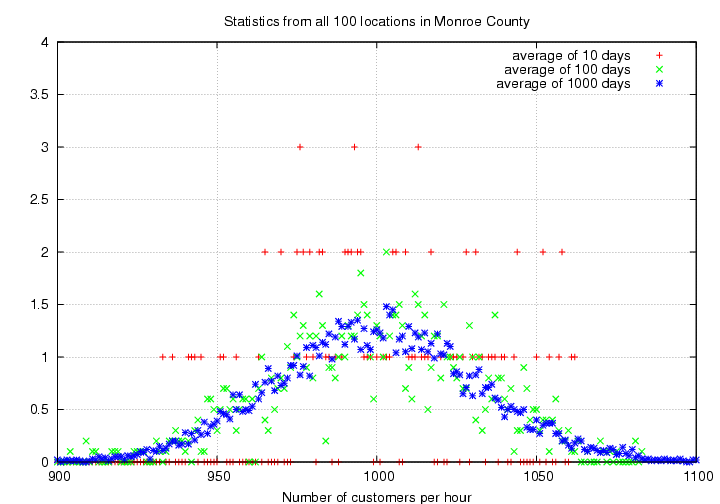
To diminish the fluctuations,
you again
extend your period of study over 10 days,
then 100 days, and take the average numbers
during each period.

Once again, the distribution becomes much
smoother and symmetric when you average over
a long period.
Exercise:
- What is the mean value of this distribution?
The standard deviation is (I again measured it)
about 32 customers per hour.
That is, the scatter around the mean value
is about +/- 32 customers.
- How does this scatter around the mean
value compare to the scatter around
the mean for a single location?
Use the raw numbers of customers
to make the comparison.
- Now, do the comparison again, but this time,
use the fractional scatter.
That is, by what percent of the average
number of customers per hour does this county-wide
measurement fluctuate?
How does that percentage compare to the
percentage scatter for a single store?
One more time --- you still need better statistics.
So, you now hire people to make
similar counts at all the restaurants in
the entire Northeastern United States.
There are N = 10,000 restaurants,
so you will find a much, much larger number of
customers per hour -- at all stores --
who pay with $20 bills.
Here are the raw counts for the first few
days of your giant study.
      Hour-by-hour counts throughout the day

  Day 1:  100115  99460  100171  100405  100621  100448  99654  99792  99892  100109
  Day 2:  100070  99780  100246  100124  99561  99764  100100  100669  100008  100209
  Day 3:  100007  99265  99960  100080  100309  100364  100183  99897  101023  99771
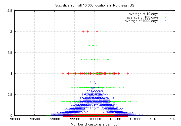
Again, you decide to use a histogram to display
this information.
And again,
you extend your period of study over 10 days,
then 100 days, and take the average numbers
during each period.

Exercise:
- What is the mean value of this distribution?
The standard deviation is this time
about 318 customers per hour.
That is, the scatter around the mean value
is about +/- 318 customers.
- How does this scatter around the mean
value compare to the scatter around
the mean for a single location,
or for N=100 locations?
Use the raw numbers of customers
to make the comparison.
- Now, do the comparison again, but this time,
use the fractional scatter.
That is, by what percent of the average
number of customers per hour does this
nation-wide
measurement fluctuate?
How does that percentage compare to the
percentage scatter for a single store,
or for N=100 stores?
The bottom line is that when you compute
the statistics of random events which occur at
some average rate,
you can make a much more
precise measurement --
in fractional terms --
when you observe a large number
of events.
The smaller the number of observed
events,
the larger (in fractional terms)
the signal will fluctuate around its
mean value.

So, even though the absolute size
of the fluctuations (or "noise")
increases with signal strength,
the fractional size of the noise
decreases with signal strength.
                                 typical fluctuation
      fractional noise      =   ---------------------
                                    mean value
We can also express this idea
in another way by taking
the inverse of this fraction:
we call that the
signal-to-noise ratio
                                     mean value
      Signal-to-noise  S/N  =   ---------------------
                                 typical fluctuation

                                     mean value
                            =   ---------------------
                                 standard deviation
When the S/N is high, we can make a very precise
measurement;
but when the S/N is low,
we can only make a rough measurement.
We'll see how this statistical property
affects our ability to measure the
brightness of a star or galaxy
in our next class meeting.
In the meantime, the
performs a somewhat more complicated version
of these same calculations
to help you estimate the S/N ratio for
a typical astronomical exposure.
For planning purposes, you might estimate
    S/N  =  1 to 5        barely detected

         =  5 to 50       fairly good measurement

         = 50 to 500      high quality measurement
Exercise:
- Use the on-line signal-to-noise calculator to estimate
the exposure time required to reach a signal-to-noise ratio
of 100 for a star of magnitude 15 in the V-band,
using our 12-inch telescope and our ST-8 CCD camera.
You can use these values for the camera on that telescope:
- pixel size 1.85 arcseconds
- FWHM = 4 arcseconds
- readout noise = 15 electrons
- aperture size = 6 arcseconds
- Use the on-line signal-to-noise calculator to find
the exposure time required to make a measurement
with a precision of 10 percent (about 0.10 magnitudes)
of a star of magnitude 18, using the ST-8 camera
on the 12-inch telescope and no filter.
For more information
 Copyright © Michael Richmond.
This work is licensed under a Creative Commons License.

 Copyright © Michael Richmond.
This work is licensed under a Creative Commons License.
