Analyzing dark frames from Sep 25, 2003

On UT Sep 25, 2003, we placed the SBIG ST-9 CCD camera onto the 16-inch telescope and acquired a set of "dark" images -- that is, images taken with the shutter closed. In theory, these images should show nothing. But in practice, dark frames do contain something: noise, due to thermal motions of silicon with the chip's lattice. In order to remove this noise from a real image, one must first understand its properties.

Today, you will

display the dark images with the tv command
define a subsection of the image with the box command
compute the mean and stdev of pixel values within the box via the mn and abx commands
create histograms of pixel values via hist
look at the histograms via xplot
figure out the mean dark current for a "warm" and "cold" camera

Getting ready

The software you'll use hasn't QUITE been set up properly on the lab computers yet. So, it will be necessary to download and install the code on the machine in front of you.

Here's what you need to do:

start a Terminal window, by clicking on the little "terminal" icon in the dock
start a browser session, by clicking on one of the browser icons in the dock
go into the Terminal window and execute the following commands, which will download some files onto your local machine. You can just cut-and-paste them, or re-type (note that it's a capital letter O)
```
         curl -O http://spiff.rit.edu/classes/phys445/code/alpha_xvista.tar

         curl -O http://spiff.rit.edu/classes/phys445/code/start_445.sh

         curl -O http://spiff.rit.edu/classes/phys445/work/data.tar
   
```
execute the following command in the Terminal to install the "xvista" package of programs and the data we need for today's class. It should cause the Terminal to print a bunch of lines that will scroll off the top.
```
         tar -xvf alpha_xvista.tar

         tar -xvf data.tar
   
```

Phew. That wasn't so bad. The next steps are ones that you will (probably) have to take, today and next week and every other time you use the Gosnell computers.

go into a Terminal window and type the following commands


         cd

         . start_445.sh

         startx

This will initialize several environment variables and then start the X11 Window System on your computer.

Use the xterm window on your display to verify that you have all the files you need for today. At the command prompt, type


         cd

         ls

You should see listings for directories called sep20_2003 and sep24_2003.

When you have reached this point, please pause, and look around. If someone nearby is having problems, please help him or her to reach this point.

Examining the dark current in images taken on Sep 24, 2003

Use the Linux cd command to change directories into the sep24_2003 directory. In that directory, you should find a bunch of raw images. Please use the ls command to verify that you have all of the following:

     dark1-001d.fit   dark10-001d.fit   dark20-001d.fit   dark30-001d.fit
     dark1-002d.fit   dark10-002d.fit   dark20-002d.fit   dark30-002d.fit
     dark1-003d.fit   dark10-003d.fit   dark20-003d.fit   dark30-003d.fit

     dark1cold-001d.fit  
     dark10cold-001d.fit 
     dark20cold-001d.fit 
     dark30cold-001d.fit

The first set, with names like dark1-, were taken with the CCD chip at a warm temperature: T = 23 Celsius. The second set, with names like dark1cold-, were taken after the chip was cooled to T = -19 Celsius.

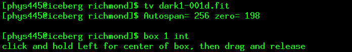
Use the tv command to display images in the "warm" series:

     dark1-001d.fit   dark10-001d.fit   dark20-001d.fit   dark30-001d.fit

What can you tell about this series of images by just looking at them, and moving the cursor around on the images?

Define a box

Display the 1-second dark image. Then type the command

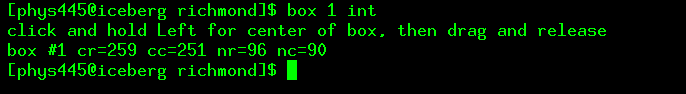
         box 1 int

You will be told to define a box by clicking and dragging ...

Make a box in the center of the image, roughly one-quarter of the image width by one-quarter of the image high. If you screw up or don't like the box you get, just repeat the command. When done, you should be told exactly where your box is:

If you now type the command

         box 1 show

the box you have just defined should appear on all open image windows. It may disappear if the window is closed and reopened, or covered and uncovered.

Boxes are useful to define subsections of images. It's often a good idea to isolate a small section of an image for statistical purposes.

Computing image statistics

There are several commands for calculating statistics of entire images, or subsections of images. The mn and abx commands produce similar information

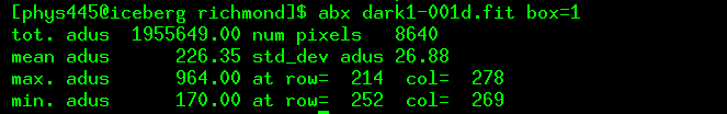
but the abx command is a bit more verbose.

Use the mn command to calculate the mean and stdev of pixel values within your box in the 1-second warm image dark1-001d.fit. Write down the result.
Repeat the measurements on other warm images: a 10-second image, a 20-second image, a 30-second image. Again, write down the results, making a small, neat table.
Plot your data on the graph paper provided. Place exposure time (in seconds) on the horizontal axis, and mean pixel value (in counts) on the vertical axis.
Determine the slope and y-intercept of the line defined by your measurements. Explain the units and meaning of the slope, and the units and meaning of the y-intercept.

When you have reached this point, please pause, and look around. If someone nearby is having problems, please help him or her to reach this point.

Making histograms of pixel values

The mean and stdev are nice, but they don't always tell the whole story. You can learn more about the properties of an image by making a histogram of pixel values; that is, finding out exactly how many pixels have a value of 100 counts, how many with 101 counts, how many with 102 counts, etc. You can use the command hist to do the job for you, like so:

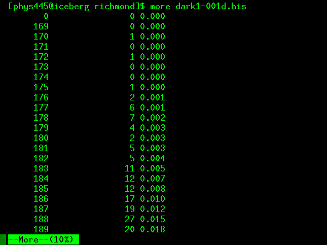
      hist dark1-001d.fit box=1

By running this command on an image, you will create a data file which has the same name as the image, but with an extension of ".his" instead of ".fit".

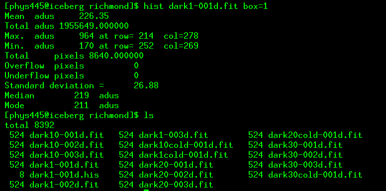
What does this ".his" file contain? A simple 2-column list of data, in which the first column represents a pixel value, and the second column the number of pixels in the image (or sub-image) which have that value. You can look at the values with the Unix command more:

But you can understand this more simply by making a graph.

The XVista package contains a quick-n-dirty plotting program called xplot. You can use it like so:

When you run the program, it should pop up a new window, inside which it should draw a graph like this:

You can quit the xplot program by typing "quit" to its command prompt.
The other way to make this graph is by using a spreadsheet program such as Excel. It will probably help to make a copy of the ".his" file with an added extension ".csv", like this:

Create a new spreadsheet, import the data values from the ".csv" file, and tell the spreadsheet to plot the pixel value on the x-axis and the number of pixels on the y-axis.

Run the hist program on one each of the 1, 10, 20, 30 second warm images
Make a graph of the distribution (using whatever software you wish)
Describe each graph. Do you see any common features?
Do the statistics "mean" and "stdev" describe this distribution accurately? Explain.

The importance of temperature

Okay, you should know quite a bit about the warm images now. The camera had a temperature of around 23 degrees Celsius during these exposures. But we also took a set of images at a temperature of around -20 degrees C. Do the images look any different?

Display side-by-side one of the 30-second warm images, and the 30-second cold image.
Aside from the mean level of each image, do you see any obvious differences in the appearance of the two images?

Is the "dark current" any different in the cold images?

Using the same box as before, measure the mean and stdev of pixel values in the 1, 10, 20, 30 second exposures of the "cold" series.
Graph these data on a second piece of graph paper
Determine the slope and y-intercept of these data
Compare the slopes and y-intercepts of the "warm" and "cold" series

Now use the hist program to examine the distribution of pixel values for the "cold" images.

What features do you see in these distributions?
Do the "warm" and "cold" distributions look similar or different? Explain.