 Copyright © Michael Richmond.
This work is licensed under a Creative Commons License.
Copyright © Michael Richmond.
This work is licensed under a Creative Commons License.
CCDs are very accurate devices: they measure linearly the amount of light which strikes them, as long as the levels remain below the saturation point. However, this can turn out to be a pain: it can reveal very small differences that might otherwise be lost in the noise. If one can make measurements to a precision of better than one percent, several systematic effects start to show themselves. One of these is due to small differences in the effective passband of different observatory systems.
So you have a bunch of measurements of the instrumental magnitude of some variable star, plus the instrumental magnitudes of some comparison stars in the field.
     CY       A       B       C
   13.079  12.592  13.670  16.075
How can we turn these instrumental magnitudes into real magnitudes?
Exercise:
- What is the best passband for these images of CY Aqr?
- What is the standard magnitude of each star (A, B, C) in that passband? (Hint: use SIMBAD or Aladin)
- What is the offset which brings instrumental to standard magnitudes?
- What is the standard magnitude of CY Aqr in the picture above?
This method is simple, quick, and will get you into the ballpark. Its results might be within 10 percent of the truth for "ordinary" objects: stars of intermediate temperature and color. But for very blue or very red stars, or objects with strange, non-blackbody spectra, it can be way off.
Astronomical observations involve a number of components:
Let's consider filters, since they usually place the strongest constraints on the detected photons. Even filters which are supposed to be identical have small differences. Below are the transmission curves of the standard Bessell V passband (which is a model for manufacturers of filters), and the "Harris V" filter at the WIYN Telescope at Kitt Peak National Observatory:
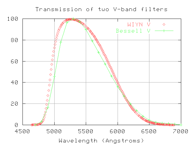
The WIYN filter is slightly broader than the standard passband. How large a difference does that make? Well, there are two ways to look at it.
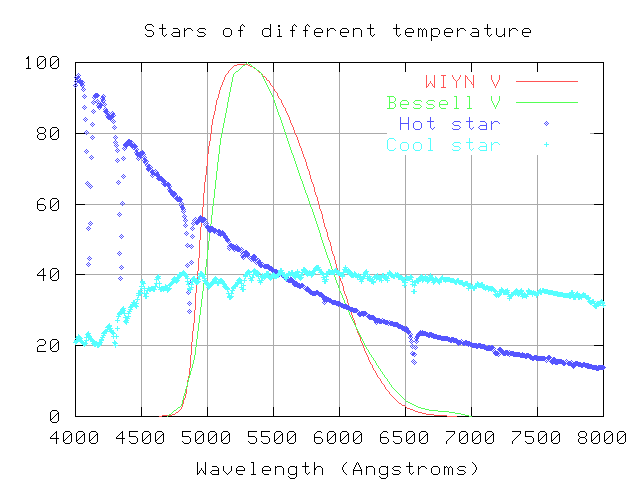
If one knows the exact shape of a star's spectrum, one can convolve the spectrum with several different passbands to predict its instrumental magnitudes. I have taken the spectra for the hot and cool stars shown on the above graph and convolved them with each of the two "V" filters. The zero point is arbitrary.
    star             Bessell V       WIYN V     (Bessell V - WIYN V)
---------------------------------------------------------------------
  A0V  (hot)          16.056        16.000           +0.056

 K0III (cool)         16.149        16.109           +0.040
Notice that the change in instrumental magnitude is NOT the same for the two stars. If I use the WIYN filter, my images will show a hot A0 star to be a bit brighter compared to a cool K0 star than it would appear through the standard Bessell filter. The difference isn't large, about 0.016 magnitudes or 1.6 percent, but it can be seen easily in good CCD photometry. There will be a similar effect for all stars of different temperatures.
How can one find out if one's system suffers from a passband mismatch? Easy: just observe a field(s) with many standard stars of known magnitudes and a range of colors (and, hence, temperatures). Then compare the measured magnitudes to the standard magnitudes, as a function of color. If a trend appears in the residuals, there's a problem.
Let's look at an example: Hwankyung Sung and Michael Bessell calibrated the 40-inch telescope and its CCD camera at the Siding Spring Observatory in Australia in the late 1990s. You can find a paper describing their work on the Astrophysics Data System Abstract Service. Searching on their names will reveal the paper Standard stars: CCD photometry, transformations and comparisons, which appeared in Publications of the Astronomical Society of Australia, vol 17, p. 244 (2000). Here's part of their Figure 3, showing the differences between the standard V-band magnitudes and their instrumental system as a function of (B-V) color.
Exercise:
- In the Siding Spring data, do blue stars appear brighter or fainter, relative to red stars, than in the standard system?
- If you pick 10 stars at random from the Siding Spring data, and compute the difference between the instrumental mag v and standard mag V, what will the typical difference be? In other words, what is the typical error in converting instrumental to standard magnitude?
- Describe a possible difference in shape between the Siding Spring V-band filter and the standard V passband which would lead to the observed effect.
Based on their data, Sung and Bessell came up with an equation which fit the mean trend in the residuals:
V = a + v + 0.072 * (B-V)
where V is the standard V-band magnitude,
a is a zero-point offset in magnitude
(i.e. a simple shift of all the magnitudes vertically
by a constant amount),
v is the measured instrumental magnitude through their "V" filter,
and (B-V) is the color of a star in the standard system.
Note that astronomers often use capital letters to denote standard magnitudes, and lower-case letters to denote the corresponding instrumental values.
The coefficient, 0.072, is an example of a first order color term. In the general form of the equation, this is usually written as b, like this:
V = a + v + b * (B-V)
Don't confuse this b with the use of "b" to denote instrumental B-band magnitudes.
Exercise:
- What are the units of the first-order color term?
- Use the data in the graph from Sung and Bessell above to estimate the value of the first-order color term b for the Siding Spring instrument.
Now, the idea is always to correct your instrumental magnitudes so that they match the standard scale. Look carefully at the equation above: in order to calculate the color correction, you need to know the standard (B-V) color of a star; but you don't know the standard V-band magnitude yet! Yikes! It looks like a circular argument. There are three ways around it:
V = a + v + b * (B-V)
into
V = a' + v + b'* (b-v)
where the values a' and b' yield the standard
magnitude in terms of the instrumental colors.
V = a + v + b * (b-v)
and make a plot of instrumental color on the x-axis versus
magnitude error (V-v) on the y-axis.
The slope of the trend line will the color term.
After Sung and Bessell make their color corrections, the residuals between their measurements and the standard V-band measurements show no systematic trend with color:
There is still some scatter, but it appears to be random. It's probably due to a combination of photon noise from the star and background.
Exercise:
- If you pick 10 stars at random from the CORRECTED Siding Spring data, and compute the difference between the instrumental mag v and standard mag V, what will the typical difference be? In other words, what is the typical error in converting CORRECTED instrumental to standard magnitude?
The best source for magnitudes of stars in the UBVRI system is a series of papers by Arlo Landolt.
The second paper contains finding charts for all the stars. Most appear in groups of three to twenty stars, in "Selected Areas" of the sky. If you observe one of these selected areas, you can acquire data on many standards all at once, which allows you to determine the color coefficients for your system in a short time. Below is a section of the chart for SA101, which is near RA 09:57, Dec 00:00.
Exercise:
- What are the exact coordinates of the star marked "363" on the chart?
- What is the V-band magnitude of that star?
I have made finding charts for a set of five fields around the celestial equator which have several stars of very different colors with well measured magnitudes.
Copyright © Michael Richmond.
This work is licensed under a Creative Commons License.