 Copyright © Michael Richmond.
This work is licensed under a Creative Commons License.
Copyright © Michael Richmond.
This work is licensed under a Creative Commons License.
When we look far beyond the Coma Cluster, we can no longer discern Cepheids or planetary nebulae or globular clusters. In our desperation, we resort to methods which have physical underpinnings which are less secure than the secondary methods. We might call them "tertiary indicators". Astronomers come up with new ideas every few years, but we'll discuss just a few of the most common ones.
Two versions of the "standard candle" idea
Need some diagrams and worked examples showing the succession of layers of an expanding SN which we see as the photospheres at different times. --- MWR 5/17/2013
Supernovae -- stars which explode violently and never recover -- come in many different varieties. One type, called Type IIP, begins the core of a red supergiant with a massive envelope of hydrogen collapses when it runs out of fuel. The outer layers of the core fall inward, then a lot of very complicated stuff happens, and the net result is
The shock wave heats the bulk of the star and accelerates it outward, to speeds far above the escape velocity. In a word, the star explodes. However, if one looks more closely, one finds that the velocities of different layers of the star vary in a systematic way: material from the inner regions has a relatively small velocity, while material from the outer regions has a relatively high velocity.
Figure taken from
Blinnikov et al., ApJ 496, 454 (1998)
The shock wave heats material up to very high temperatures, well over 100,000 Kelvin, ionizing all the hydrogen. The outermost layers emit X-rays and UV for several hours after the shock breaks out of the star, but then cool off quickly. When the temperature of the gas falls to roughly 6000 Kelvin, however, the hydrogen begins to recombine. At this point, as the outermost layer switches from ionized to neutral, its opacity drops: neutral hydrogen gas is MUCH more transparent than ionized gas.
When the outermost layer recombines, it becomes essentially transparent, and we can see into the layer below it. This layer is still hot enough that hydrogen is ionized ... but within a short time, it, too, cools off to about 6000 Kelvin and recombines. When it becomes transparent, we can then see into the NEXT layer of the star, and so on and so on.
The important facts here are
As time goes by, and we see further into the star, the velocity of this special layer will decrease. The graph below shows the evolution of a computer model of a Type II supernova -- the lines are drawn at roughly one-week intervals.
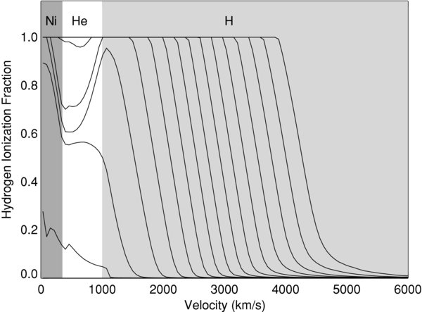
Figure taken from
Kasen and Woosley, ApJ 703, 2205 (2009)
The solid curve in the figure below shows the evolution of a computer model of an exploding star, while the circles show measurements of real supernovae.
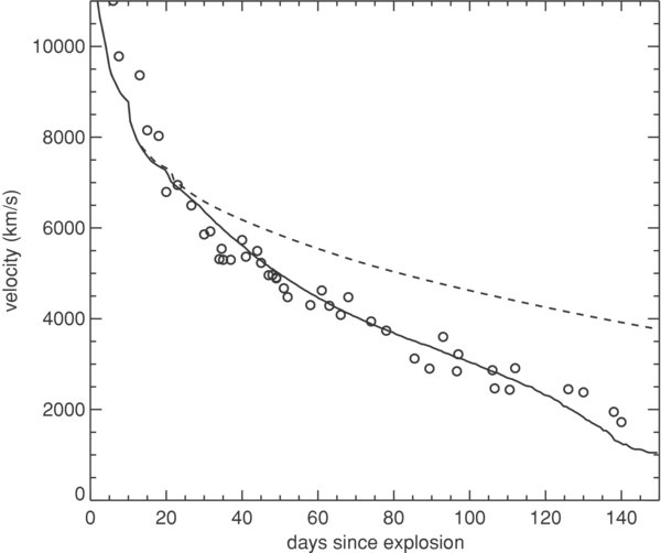
Figure taken from
Kasen and Woosley, ApJ 703, 2205 (2009)
The radius of the photosphere at some time t can be written as
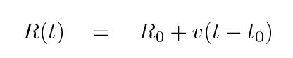
where t0 is the time of explosion and R0 is the radius at the time of explosion. With high-quality spectra of the supernova, we can measure the velocity of the photosphere at different times.
Because the photosphere is in such a simple condition -- nearly pure hydrogen, at a temperature close to 6000 K -- it isn't too difficult to compute the radiation it emits. To first order, the photosphere acts like a "dilute blackbody", emitting flux
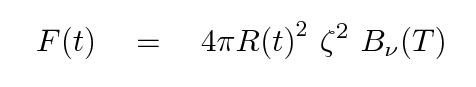
where T is the temperature ~ 6000 K, and ζ is a "dilution factor", inserted into the ordinary blackbody equation to account for several factors which cause the spectrum of the actual star to differ from that of a perfect blackbody.
Using spectroscopy and photometry, we can measure v(t) and the observed flux f(t). If we make measurements at several different times, when the photosphere has different sizes and luminosities, we have enough information to solve for the time of explosion, initial size of the star, and determine the distance as well; it's just a matter of comparing the luminosity F(t) to the observed flux f(t) and using the inverse square law (and hoping that there was no extinction, etc.).
It is a nice coincidence that the speed with which the recombination wave runs deeper into the star is very roughly the same as the rate at which the star is expanding; in other words, the radius of the apparent photosphere doesn't change a great deal while the wave is still moving through the envelope. As a result, the luminosity of Type IIP supernovae hits a plateau (hence the "P") and remains nearly constant for a month or two.
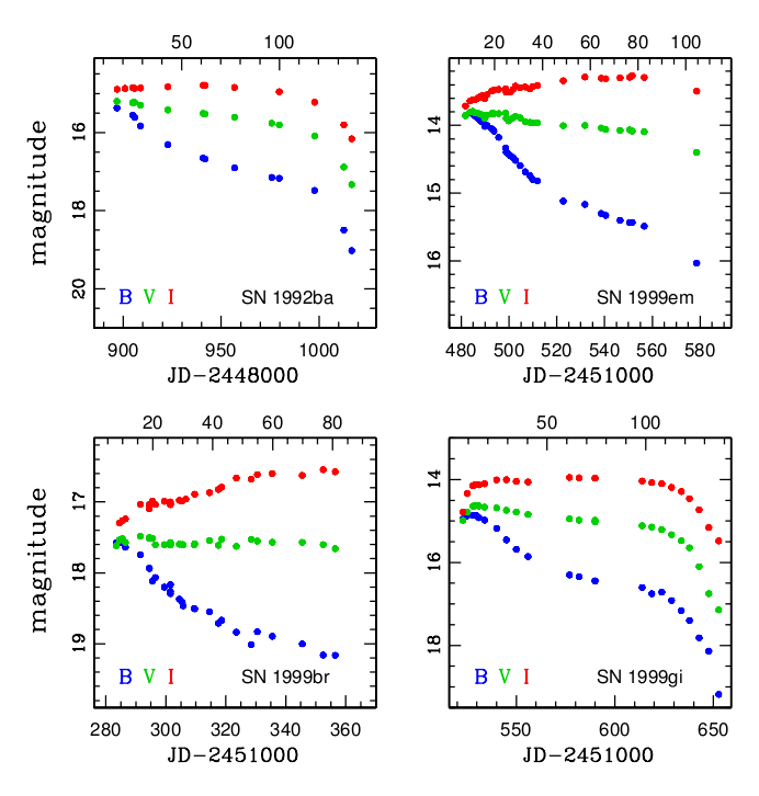
Figure taken from
Jones and Hamuy, RMxAC, 35, 310 (2009)
As an example of the technique, consider the galaxy M51, in which two Type II supernovae have exploded in the past decade: SN 2005cs
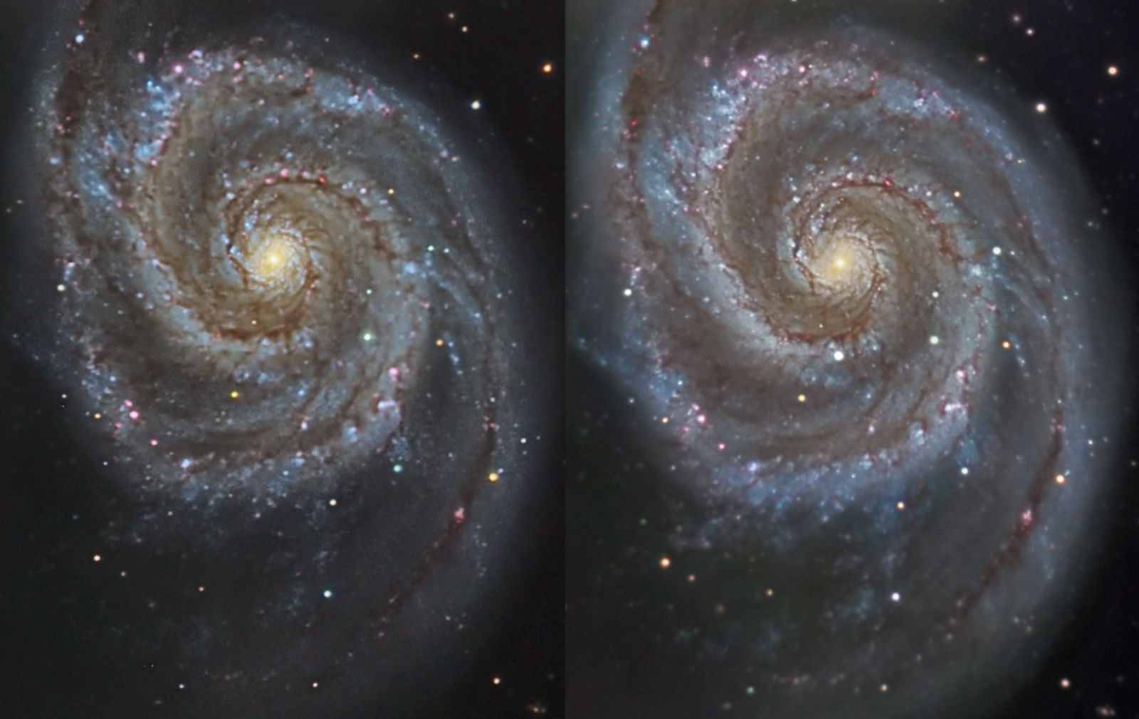
Image copyright
R Jay GaBany . Thanks to
Astronomy Picture of the Day.
and, six years later, SN 2011dh
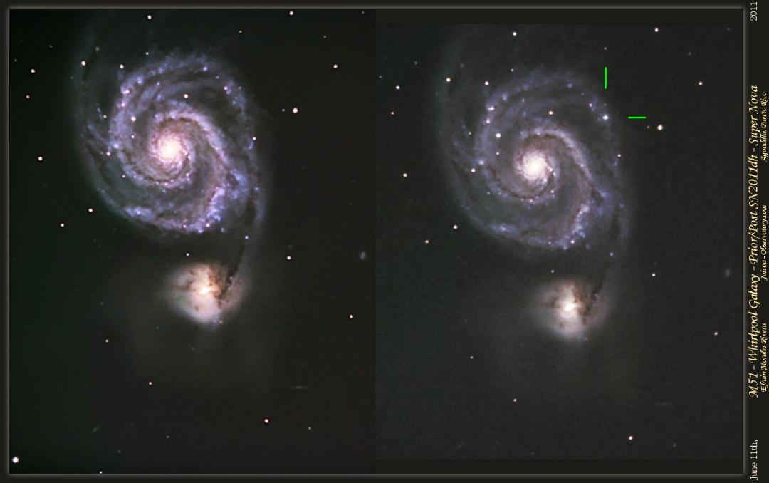
Image courtesy of Efrain Morales Rivera of the
Jaicoa Observatory
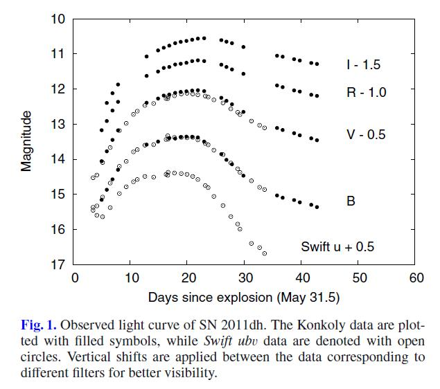
With a combination of light curves (left) and spectra (right), Vinko et al., A&A, 540, 93 (2012) were able to apply the expanding photosphere method to both supernovae.

Figures taken from
Vinko et al., A&A, 540, 93 (2012)
The authors were able to estimate for each supernova
The table below shows their values for these parameters for SN 2005cs; the paper includes similar calculations for SN 2011dh.
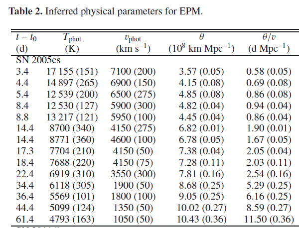
Table taken from
Vinko et al., A&A, 540, 93 (2012)
Putting together all the information, one can compute the distance to the supernova (and hence its host galaxy, M51) for each epoch of measurements for each event.
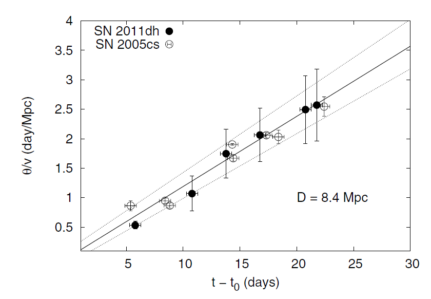
Figure taken from
Vinko et al., A&A, 540, 93 (2012)
We can apply this technique to large distances, because Type IIP SNe are very luminous: their typical absolute magntiudes are between -15 and -18.
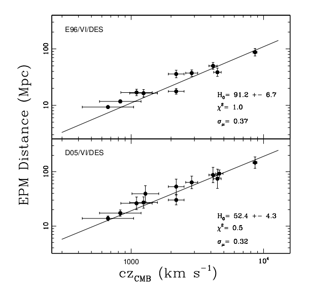
Figure taken from
Jones and Hamuy, RMxAC, 35, 310 (2009)
  Q:  How distant are the Type IIP SNe
      used in the figure above?


      How does that compare to the distance
      to the Virgo Cluster?


      What is the distance modulus to the
      most distant event in the figure?
How precise is this method? The best cases yield an uncertainty in distance of around 12-15 percent.
  Q:  If the uncertainty in distance is
      15 percent, what is the uncertainty
      in distance modulus?
Type Ia supernovae have little in common with Type IIP supernovae, apart from the fact that both involve titanic explosions which destroy stars. The progenitor of a Type Ia SN is not a giant, bloated, massive young star; instead, it's the very opposite: a tiny, compact, not-very-massive white dwarf. But not just any white dwarf: a white dwarf in just the right sort of binary system.

Image copyright
David Hardy
If a white dwarf accretes material at just the right rate, a layer of accreted material can accumulate at the surface. If the total mass of the white dwarf approaches a critical value, the Chandrasekhar limit -- about 1.4 solar masses -- then conditions at the center (or perhaps slightly to one side of the center) of the star allow thermonuclear reactions to take place. Specifically, the carbon which makes up much of of the white dwarf's core can begin to fuse into heavier elements.
This fusion releases energy, which heats up the core. Because the core is degenerate, however, it does not expand and cool, but simply remains at its original size. The increased temperature then promotes further fusion, which increases the temperature even more, and a runaway thermonuclear reaction occurs.
BOOM!
The resulting explosion creates a fireball which can outshine its entire galaxy for a few weeks.
Now, back in the Old Days, SNe Ia were used as standard candles: each was assumed to have exactly the same absolute magnitude, and so the apparent magnitude would yield the distance. However, as astronomers accumulated better measurements and larger samples, it became clear that SNe Ia are not all identical. These supernovae appear to vary in a systematic way.
For example, if we measure the amount by which supernovae decline in brightness 15 days after maximum light in the B-band,

Figure taken from
Richmond et al., AJ 111, 327 (1996)
and compare it to the absolute magnitude of the event, we find a clear correlation.

Figure taken from
Hamuy et al., AJ 112, 2391 (1996)
    Superluminous        Normal          Subluminous
 -----------------------------------------------------

     decline slowly                     decline quickly

     bluer                              redder

     faster ejecta                      slower ejecta

 -----------------------------------------------------
If we can measure enough SNe Ia to pin down these relationships between absolute magnitude and other observable quantities, we can perhaps turn SNe Ia into standard-izable candles; not as nice as truly standard candles, but still useful. There are several groups working on this problem, with slightly different techniques, and both have found some success. The SALT procedure involves choosing one of a set of templates which best fits the light curve of some particular observed SN Ia.
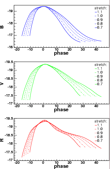
Figure taken from
Guy et al., A&A 443, 781 (2005)
Using these methods to correct for the relationship between decline rate and luminosity, one can reduce the uncertainty in distance modulus measurements for SNe Ia to perhaps 0.15 magnitudes.
  Q:  If the uncertainty in distance modulus
      is +/- 0.15 magnitudes, what is the
      uncertainty in distance?

      Express as a percentage.
If one looks at SNe in the near-infrared H-band, they may indeed be nearly identical; the Hubble diagram below uses measurements which have NOT been corrected for the decline-rate effect. To be fair, much less work has been done in the near-IR than in the optical.
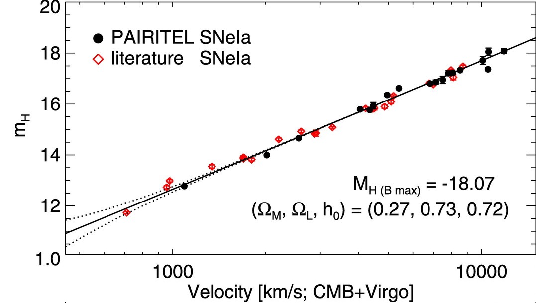
Figure taken from
Wood-Vasey et al., ApJ 689, 377 (2008)
One of the reasons astronomers spend so much time trying to understand Type Ia SNe is that they are really, really luminous: their absolute magnitudes are around -19 or -20! That means that they can be seen at VERY large distances, which means that they may be able to test different cosmological models.
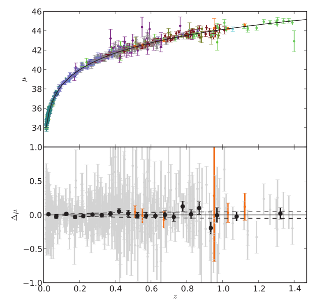
Figure taken from
Amanullah et al., ApJ 716, 712 (2010)
  Q:  What is the largest redshift out to which
      SNe Ia have been detected, as shown in
      the figure above?


      What is the distance modulus to that
      location?  Just look at vertical axis.


      To what (luminosity) distance, in Mpc, does that
      correspond?

         If you have a network device,
         go to Ned Wright's Cosmology Calculator
         and look it up.

         If you don't, use the definition
         of distance modulus.
Actually, the record for "most distant supernova" is broken every few years. The current (April 2013) holder is SN UDS10Wil, discovered during the course of the CANDELS survey with HST.
You have to be very, very careful to find objects at this distance. The supernova fell within the light of its host galaxy, and was found only via an image-subtraction technique. Note the scale bar at right.
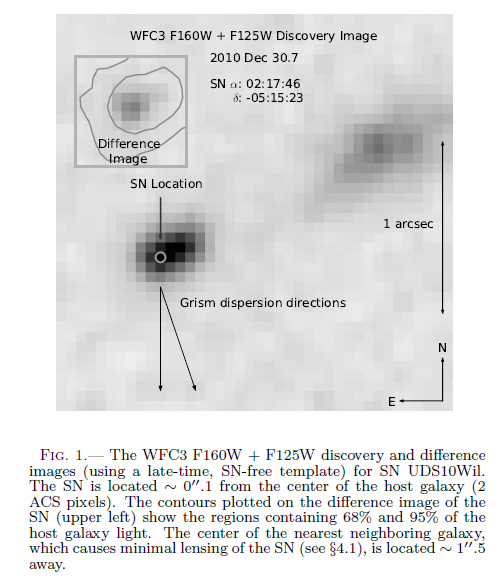
Figure taken from
The Discovery of the Most Distant Known Type Ia Supernova
at Redshift 1.914
by Jones et al., ApJ (2013)
The spectrum of this object is all mixed up with that of its host galaxy, as the figure below shows. The sharp emission line in the host-subtracted spectrum (the panel at upper left) is a residual of the very strong [O III] 5007 emission line of the host, not part of the supernova's spectrum. Look at the right-hand panels for a closeup of the real SN features -- such as they are.

Figure taken from
The Discovery of the Most Distant Known Type Ia Supernova
at Redshift 1.914
by Jones et al., ApJ (2013)
The light curve doesn't include all that many measurements, and we did not measure the light exactly at the peak time. So, determining the "peak magnitude" is a difficult job.
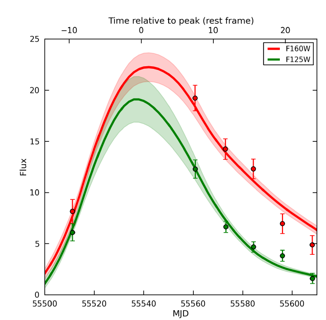
Figure taken from
The Discovery of the Most Distant Known Type Ia Supernova
at Redshift 1.914
by Jones et al., ApJ (2013)
Sometimes, even type Ia SNe aren't bright enough. If you want to measure distances out to REALLY high redshifts, like 2 or 3 or 5, then you need to find a distance indicator which is more luminous than all the stars in an ordinary galaxy. How about -- all the stars in the brightest galaxy in an entire cluster?
Why should the brightest member of cluster A have the same luminosity as the brightest member of cluster B?
I have no idea.
Still, it's easy enough to do, so why not give it a try?
The idea is a pretty old one.
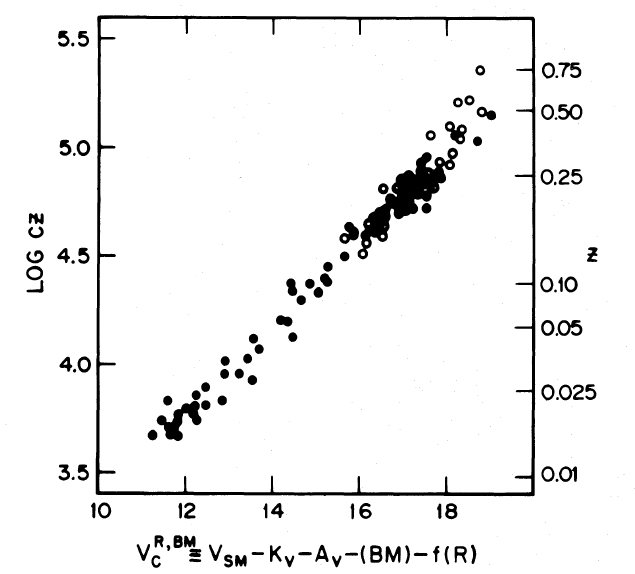
Figure taken from
Kristian, Sandage and Westphal, ApJ 221, 383 (1978)
How well do BCGs work as standard candles? Collins and Mann, MNRAS 297, 128 (1998) find that a sample of BCGs in a set of clusters with high X-ray luminosities have a scatter of about 0.22 magnitudes in K-band.
One of the really big problems with this method is that BCGs are made up of stars, and stars do evolve over time. If we look at BCGs at high redshift, we are seeing the light they emitted in the past. It is not only possible, but certain, that evolution of the stellar population has occurred. Therefore, when we compare nearby and distant BCGs, we can NOT expect them to be identical.
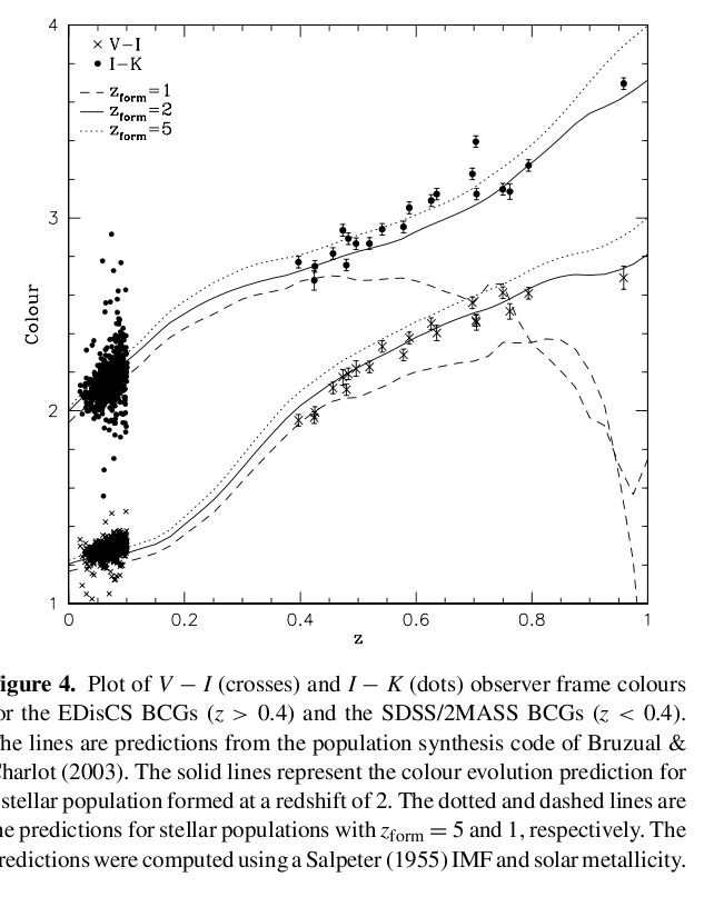
Figure taken from
Whiley et al., MNRAS 387, 1253 (2008)
  Q:  One particular BCG from Collins and Mann
      has a distance of about 5200 Mpc and
      an apparent K-band magnitude of 16.14.

      What is the absolute K-band magnitude
      of this galaxy?
Note that absolute magnitudes in optical bands may be somewhat different, but they are still more luminous than any other distance indicator.
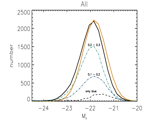
Figure taken from
Pipino et al., arXiv 1011.3017 (2010)
Whiley et al., MNRAS 387, 1253 (2008)
James and Mobasher, MNRAS 317, 259 (2000)
Wen and Han, arXiv 1104.1667 (2011)
Loubser et al., MNRAS 391, 1009 (2008)
Aragon-Salamanca, Baugh and Kauffmann, MNRAS 297, 427 (1998)
Copyright © Michael Richmond.
This work is licensed under a Creative Commons License.