Copyright © Michael Richmond.
This work is licensed under a Creative Commons License.
Copyright © Michael Richmond.
This work is licensed under a Creative Commons License.
This is a bit of a cheat. Cepheids might be classified as more secure and reliable than the other distance indicators in today's lecture. After all, each Cepheid is just a single star, and astronomers have had many years of practice to create accurate models of the physics inside a star. We can observe Cepheids within our own Milky Way, as well as in the LMC, so it is possible to measure distances to some Cepheids using very accurate parallax methods (and many more Cepheids once GAIA has been launched).
However, since Cepheids can be used -- with some difficulty -- to determine distances to some of the nearby clusters of galaxies, it's fair to list them here. Below are a couple of examples.
This is no easy task. In galaxies as distant as the Virgo Cluster, even the brightest Cepheids are close to the limit of detection. Moreover, each pixel of any camera will subtend such a large area on the sky that it will blend together the light of the Cepheid with that of many other stars in the host galaxy.
  Q:  The PSF of a space telescope has a FWHM of about
      0.15 arcseconds.  It takes pictures of a galaxy
      in the Virgo cluster, about 20 Mpc away.

      What is the diameter of that PSF projected onto the
      galaxy?  Express your answer in parsecs.


  Q:  Light from an extended region around each Cepheid
      is mixed with light from the Cepheid itself.

      How does this change the measurement of the
      Cepheid's magnitude?

      How does this change our estimate of the
      distance to the Cepheid?
This is no easy task. Consider the case of NGC 4548 in the Virgo Cluster. The stars in question are pretty close to the limit of detection, as these sample images show:

Figure taken from
Graham et al., ApJ 516, 626 (1999)
The light curves are nonetheless pretty convincing:

Figure taken from
Graham et al., ApJ 516, 626 (1999)
The period-luminosity relationship is consistent with the expected one, though the scatter is indeed large. Some of this is due to the measurements, and some due to the range of properties of Cepheids with a given period.
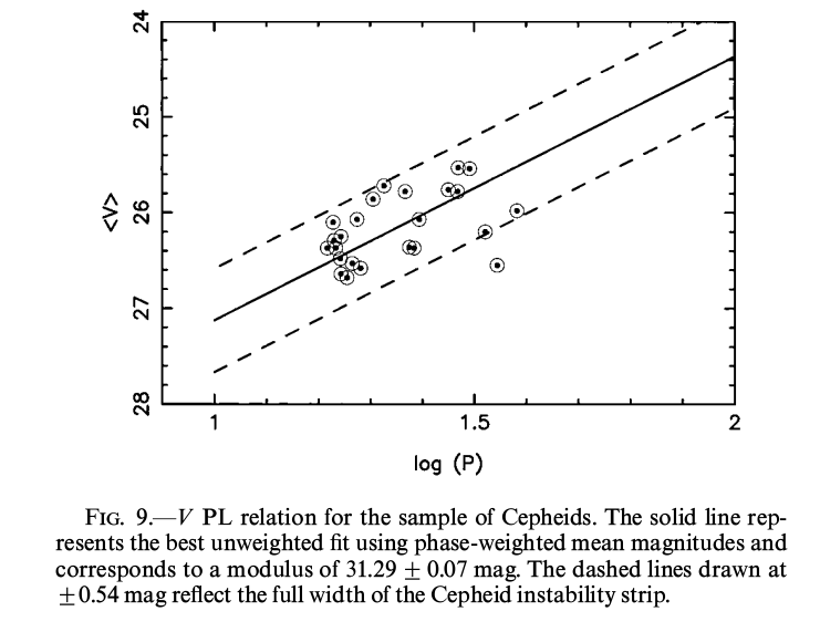
Figure taken from
Graham et al., ApJ 516, 626 (1999)
  Q:  Pick one of the illustrated light curves.
      Using the relationship

        <V>  =  -2.76 log(P)  -  1.40


      determine the distance to your Cepheid.
In the next few years, we may see a Cepheid measurement to galaxies in the Coma Cluster!
We now enter a new regime of distance indicator: the "luminosity function" technique. The basic idea is:
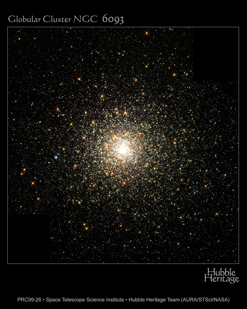
The first example of this type of indicator is the luminosity function of globular clusters. You know what globular clusters are, right? Here's an example of one which orbits the Milky Way:
When we look at (most) other galaxies, however, we can't resolve the individual stars in the clusters. Instead, we see a single tiny ball of light; at the distance of Virgo, an entire cluster can just barely be distinguished from a point source.

Figure taken from
Jordan et al., ApJS 154, 509 (2004)
Three clusters of data points can be clearly identified: (1) a group of unresolved sources with rh ~ 0, which correspond mainly to foreground stars; (2) a diagonal swath of points with faint magnitudes and large sizes, which correspond mainly to background galaxies; and (3) a group at z850 ~ 20-25 and rh ~ 3 pc, which correspond mainly to bona fide GCs.
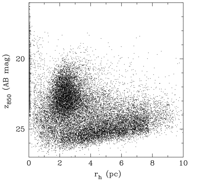
Figure taken from
Jordan et al., ApJS 180, 54 (2009)
Now, globular clusters are NOT identical: some are much larger than others, some are much more luminous than others. If we count the number of clusters in the Milky Way as a function of their absolute magnitudes, we find a roughly gaussian distribution. Yes, there's a tail at the low-luminosity end; no, for our purposes, that's not very important (why not?).
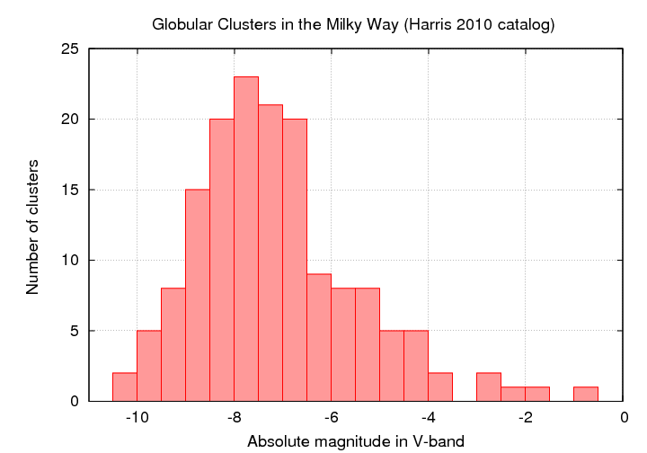
Figure based on data from
http://physwww.mcmaster.ca/~harris/mwgc.dat
If we look at the distribution of apparent magnitudes of globular clusters around other galaxies, we see something like a gaussian distribution (well, sometimes ... more on that in a moment). In the figure below, the left-hand panels show histograms of the GCs in a pair of Virgo Cluster galaxies.
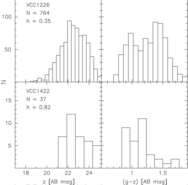
Figure taken from
Jordan et al., ApJS 180, 54 (2009)
The right-hand panels in the figure above show a histogram of the COLORS of the GCs around those two Virgo galaxies. It seems that GCs come in two flavors, "red" and "blue"; the difference has something to do with metallicity. Is the mixture of flavors the same in all galaxies? Does it matter for the use of GCLF as a distance indicator? Good questions.
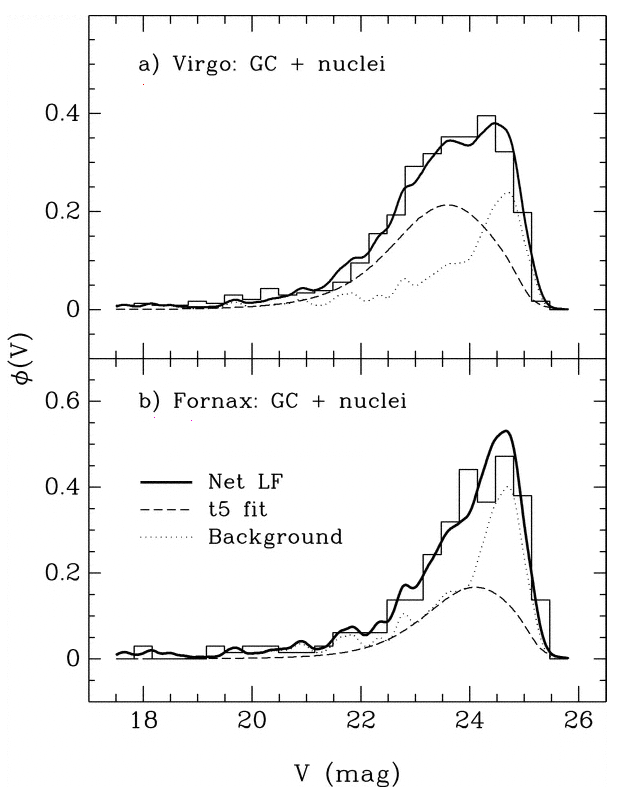
Figure taken from
Miller and Lotz, ApJ 670, 1074 (2007)
  Q:  Choose either the Virgo or the Fornax
      distribution.  Compare it to the
      distribution of Milky Way GC absolute
      magnitudes.  Use it to estimate the
      distance to the Virgo or Fornax galaxy
      cluster.
A digression on the dangers of incompleteness
Let's go back and take a closer look at that last graph. It showed histograms of the observed luminosity functions of GCs in the Virgo and Fornax clusters. Concentrate on the lower panel. Is the model of the luminosity function, shown in the long dashed line, really symmetric?
Figure taken from Miller and Lotz, ApJ 670, 1074 (2007)No. It isn't symmetric. There are more clusters on the "bright" side of the apparent peak, and fewer clusters on the "faint" side.
  Q:  Why should the observed histogram show
      more clusters on the bright side of the peak?
The answer is pretty simple: bright objects are easier to detect! If you are looking for stars or clusters or galaxies or just about any sort of object in an astronomical image, you generally have a better chance of finding the bright items than the fainter ones. Pretty obvious, really.
The trouble is -- this introduces a systematic bias, or selection effect, into any analysis based on the detected objects. Depending on the particular sort of analysis, this sort of selection effect might be insignificant, or it might be very important.
  Q:  In this case, we are matching the peak
      apparent magnitude of the GCLF in Fornax
      to the peak absolute magnitude of the
      GCLF in the Milky Way.

      If we do NOT take the selection effect
      into account, what will happen to the
      distance modulus we compute?
Let's consider a second example. Suppose that we are interested in open star clusters, and we are making a catalog which contains the size of each cluster. We take a picture of the cluster Perseus 3 and see the pattern of stars below. The scale bar is marked in arcseconds.
Q: What is the radius of the cluster?

A few years later, another astronomer is granted time on a bigger telescope and takes a series of exposures of Perseus 3 with a range of exposure times. Click on the picture above to see the results of his work.
Q: What is the radius of the cluster?So, how can we deal with this menace to quantitative measurements? We must counter-attack with a quantitative correction for the effects of the varying degree of completeness. What we need is a way to describe the probability that an object is detected as a function of its magnitude. Not as simple as
- bright: probably detected
- faint: probably missed
but more sophisticated, like this:
- mag < 22.0: 95% chance of detection
- 22 < mag < 23.0: 75% chance of detection
- 23 < mag < 24.0: 50% chance of detection
- 24 < mag < 25.0: 15% chance of detection
- 25 < mag : 0% chance of detection
If someone else has studied this particular region of the sky with a bigger telescope some time in the past, and published a detailed catalog of the objects in the area, then we can compare that catalog to the objects in our study to make this sort of table.
Alas, in most cases, there is no pre-existing deep catalog of objects in the area which one is examining.
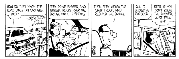
  Q:  How can we make any accurate statements
      about the probability of detection if don't
      really know what we ought to be seeing?
In the "old days", this was a tough problem. Since we have these newfangled devices called computers, however, there is a straightforward procedure we can follow to get a good, quantitative measure of incompleteness. The following Calvin and Hobbes comic strip may give you a clue ...
Start with some image showing the region of interest. This is a portion of the XMM-Newton/Subaru Deep Field.
Use some tool to find and measure the properties of all the objects in the image.
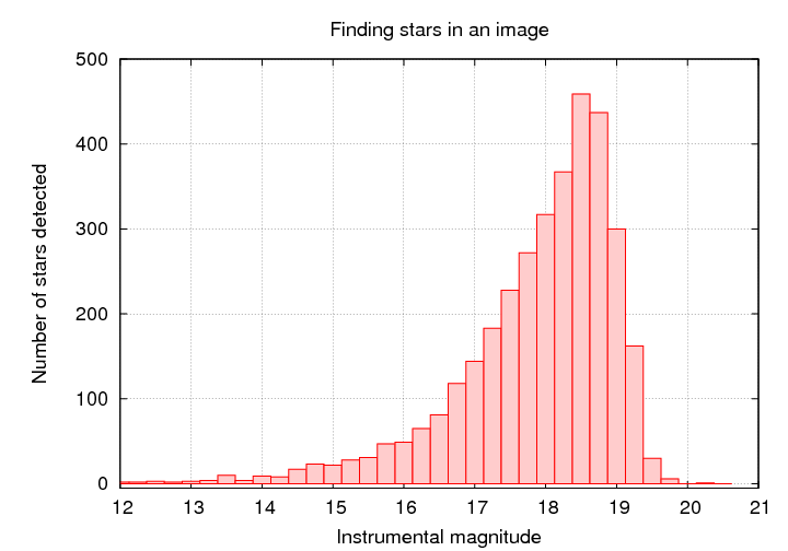
   Q:  At what magnitude do you think
       we fail to detect stars?
Now, the tricky part: use some tool to generate a set of fake objects, with the same size and shape as real objects, at random locations. Add those fake objects to the original image.

It's pretty easy to see the fake stars in the image above, isn't it? Try an image with fainter fake stars ...

Run this synthetic image, with real and fake objects, through your object-finding tool. Compare the list of objects found to the list of fake stars added. Compute the fraction of all the fake objects which were actually detected by your software.
Repeat for fake objects covering a wide range of magnitudes.
You can then make quantitative statements about the fraction of REAL objects which were (probably) detected by your software.
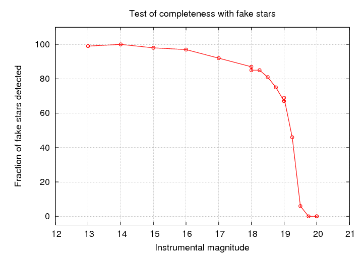
The point at which the fraction of objects detected falls to 50% is commonly used to define the completeness limit or plate limit. You must be very, very careful if you attempt to use measurements which are close to, or -- heavens above! -- beyond the completeness limit.
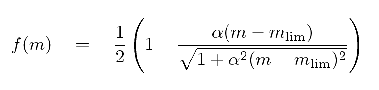
Fleming et al., AJ 109, 1044 provides a nice little analytic function which may work well to model the fraction of objects detected as a function of magnitude.
That function makes a gentle "sigmoid-ish" transition from 1.0 to 0.0 over a range which can be adjusted by the parameter α. It's similar to the shape seen in, for example, the case of stars in the XMM-Subaru Deep Survey.
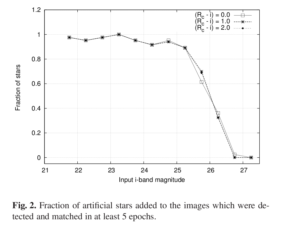
Figure taken from Richmond et al., PASJ 62, 91 (2010)
Planetary nebulae (PNe) are formed when an old star gently blows off its outer layers and then ionizes the shell of gas.
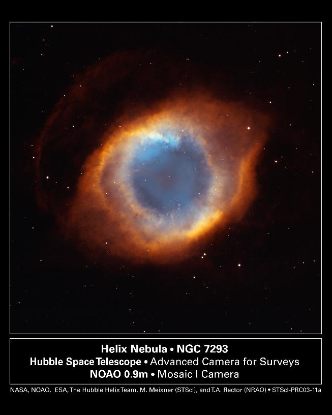
Image courtesy of
NASA, NOAO, ESA, the Hubble Helix Nebula Team, M. Meixner (STScI), and T.A. Rector (NRAO).
The ionized gas emits very strong emission lines, especially H-alpha, [NII] 6584, and the [OIII] 5007 complex.
Figure taken from
Magrini et al., A&A 443, 115 (2005)
Because PNe emit a large fraction of their total energy in a few narrow emission lines, it is easy to pick them out in a crowded field, even if they are unresolved. One technique involves slitless spectroscopy.

Figure taken from
Merrett et al., MNRAS 369, 120 (2006)
Some planetary nebulae are more luminous than others for various reasons: the underlying hot core may emit more or fewer ionizing photons, the shell of gas may be more or less dense, and so forth. In general, there only a few powerful PNe, but many weak ones. The distribution of PNe luminosities isn't a gaussian, but a sort of power law which just falls off at the bright end.
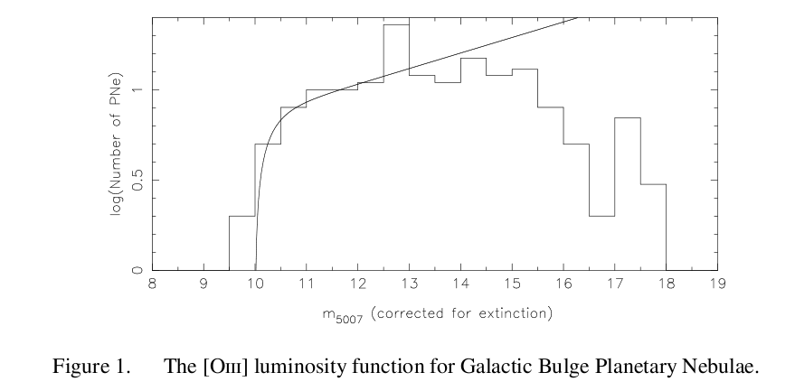
Figure taken from
Kovacevic et al., Asymmetric Planetary Nebulae 5 conference, 2011
"Hey!," you shout, "that distribution DID look sort of gaussian." Of course, what you see is not always an accurate representation of some underlying population. For example, if one looks ALL OVER the galaxy M31 for planetary nebula, and measures the apparent brightness of each one, the luminosity function turns over at the faint end.

Figure taken from
Ciardullo et al., ApJ 339, 53 (1989)
On the other hand, if one looks only in portions of the galaxy which are relatively free of dust, and counts those planetary nebulae, one finds a very different shape for the luminosity function:
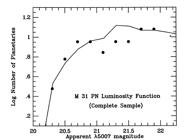
Figure taken from
Ciardullo et al., ApJ 339, 53 (1989)
Ciardullo et al., ApJ 629, 499 (2005) find that one can describe the shape of the PNLF with a function of the form
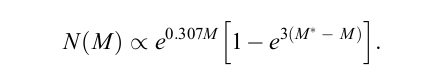
where M expresses the flux of the PN's light in the OIII 5007 emission line, using the flux of that line in ergs per sq. cm. per second, like so:
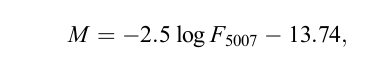
and M* is the absolute magnitude of the brightest PN in some population; that is, the magnitude it would have if placed at a distance of 10 pc. Ciardullo et al. find that the value of the most luminous planetary nebula in a number of relatively nearby galaxies is just about the same: M* = -4.47 +/- 0.05 .
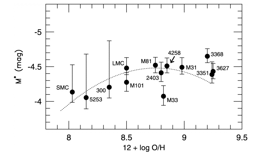
Figure taken from
Ciardullo et al., ApJ 577, 31 (2002).
  Q:  How many ergs per sq. cm. per second
      would we receive from a PN with
      M*, if it were placed at the
      standard distance of 10 pc?


  Q:  What is the luminosity, ergs per second,
      that this object is emitting in the
      OIII line?


  Q:  How does this luminosity, in OIII alone,
      compare to the luminosity of the Sun
      at all wavelengths?
So, how can we use PNe to determine distances? It's similar to the method we used for the GCLF:
Consider this set of PNLF.
Figure taken from
Ciardullo et al., ApJ 577, 31 (2002).
  Q:  NGC 2403 is at a distance of about
      3.1 Mpc from the Earth.

      Choose one other galaxy in this set.
      Determine its distance using the
      PNLF.
This technique was invented pretty recently; it was first described by Tonry and Schneider, AJ 96, 807 (1988). The basic idea is to use the "graininess" in an image which contains many stars all blended together to estimate the number of stars per resolution element. In one knows the number of stars per square pc in the stellar population, then one can use the ratio to determine the size of the resolution element in pc, and so the distance to the galaxy.
It's similar to the way that a halftone photograph like this

appears to be smooth shades of gray, when seen from a distance, but breaks up into discrete dots of black and white when one comes closer.
![]()

Let's consider a simple situation: a one-dimensional "galaxy" made up of bar-shaped "stars". If the galaxy is close enough, we can resolve the individual "stars", so that each one is separated from its neighbors by empty, black space.
 Note the high contrast
If the galaxy is ten times farther away, then the stars begin to blend together. The average pixel now contains light from one star (appearing light grey), but due to the random location of stars, a few pixels are still empty (black), and a few pixels contain the combined light of several stars (bright white).
 No longer pure black vs. pure white
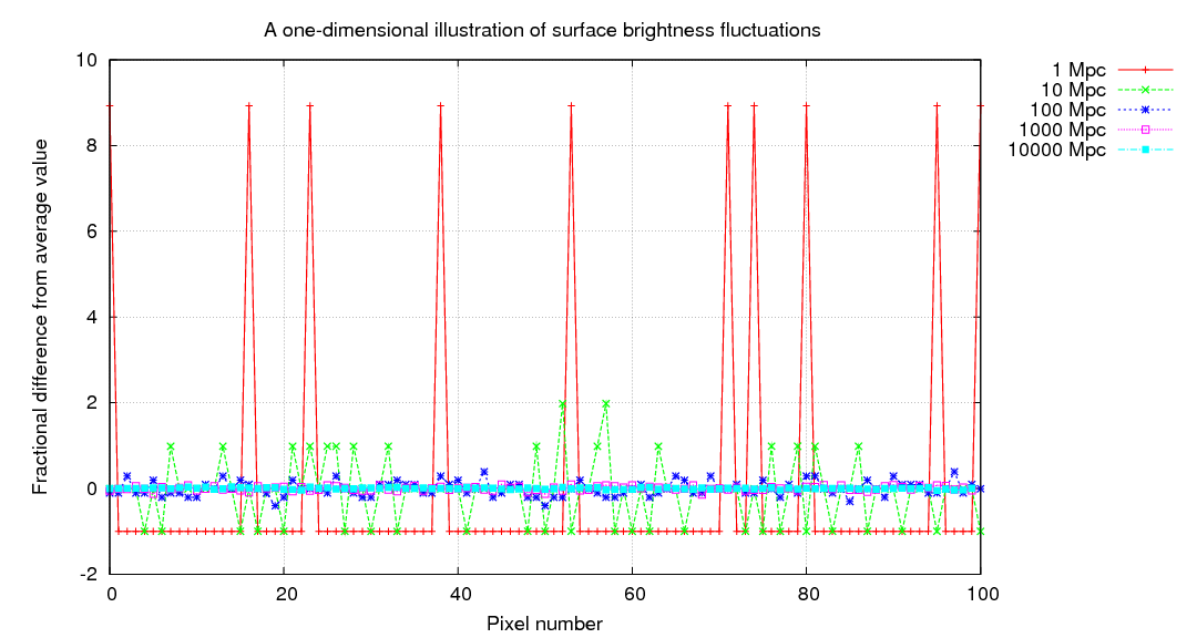
If we move a single galaxy farther and farther away, the average pixel contains a blend of light due to a larger and larger number of stars; as a result, the range of pixel values decreases, since the size of the random fluctuations decreases as we add together more and more stars. In the figure below, the gold bars show how the entire image at 1 Mpc is compressed into the first 10 pixels of the image at 10 Mpc, the entire image at 10 Mpc is compressed into the first 10 pixels of the image at 100 Mpc, and so forth.
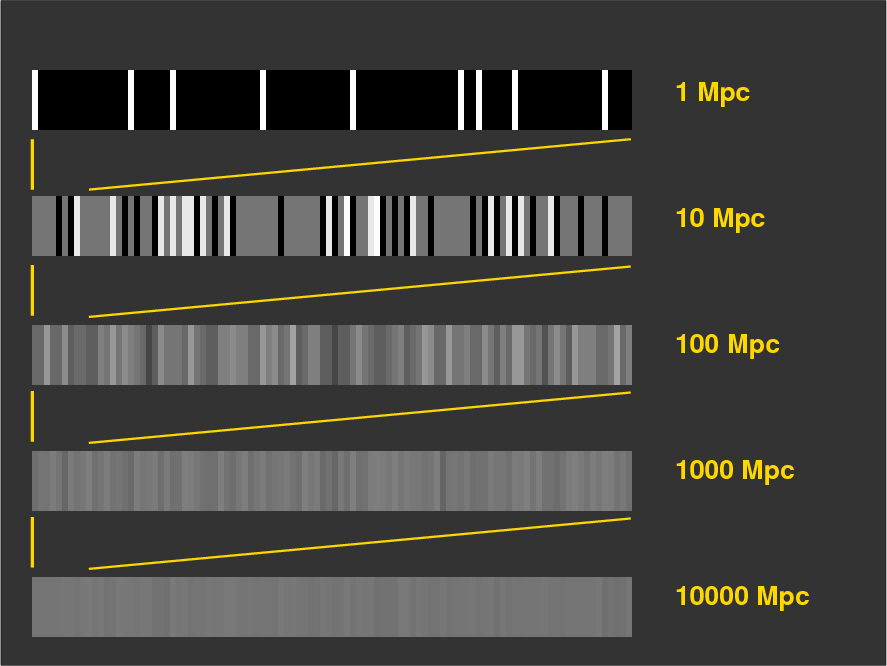
The pattern is clear:
Let's quantify these statements. In the synthetic one-dimensional "galaxies", there is an average of 1 star for every 10 pixels when viewed from 1 Mpc. If every star has an identical intensity of 1 unit, then the average pixel value must be 0.1.
When we view this "galaxy" from a distance of 10 Mpc, each pixel now contains 10 times as many stars. I've scaled the intensities so that the average value is still 0.1, but you can see that the changes from one pixel to the next are now much smaller. If you click on the picture, you'll see the progression as we move the galaxy from 1 Mpc to 10000 Mpc.

We can be even more quantitative by computing the fractional difference from the average pixel value, on a pixel-by-pixel basis. If a galaxy is close to us, this fractional difference can be very large, but it shrinks rapidly with distance.
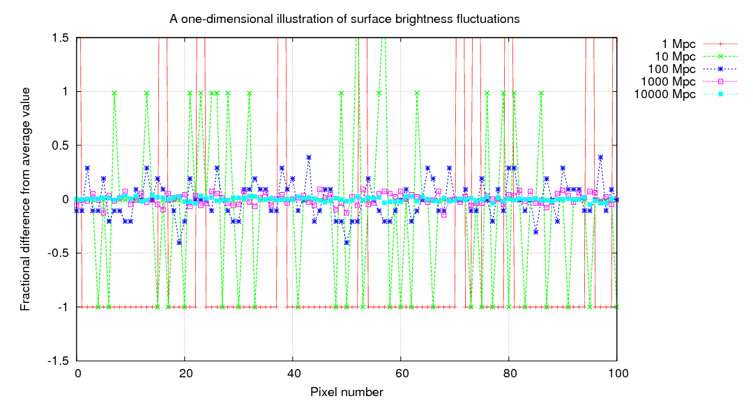
As one might expect, there's a simple relationship between the distance of the galaxy and the typical size of these deviations from the average pixel value.
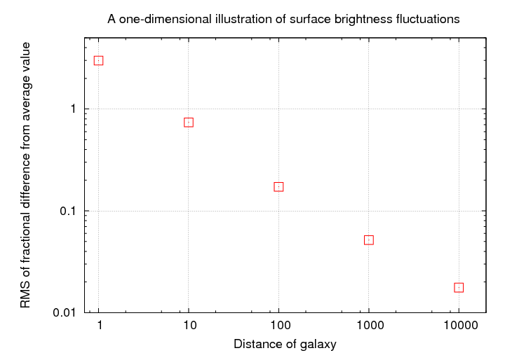
One could use this relationship to determine distances in the following way:
Now, in the real world, with its three-dimensional galaxies consisting of billions of stars drawn from heterogeneous populations, the problem is much more complicated; but the basic idea is the same.
You can see an example of the fluctuations in this side-by-side comparison of a Virgo-cluster galaxy (on the left) and the residuals after a smooth model of the galaxy has been subtracted (on the right).
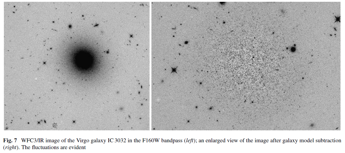
Figure 7 of
Blakeslee, J. P., ApSS 341, 179 (2012)
One way to measure quantitatively the size of the fluctuations in a galaxy's light is to take the Fourier transform of a two-dimensional image. If the galaxy is nearby, then the power of those fluctuations (the amplitude of the curved line in the diagram below) will be large:

Figure taken from
Tonry and Schneider, AJ 96, 807 (1988).
If the galaxy is distant, then the power of those fluctuations will be small:

Figure taken from
Tonry and Schneider, AJ 96, 807 (1988).
The literature on SBF often uses the notion of the "fluctuation magnitude", denoted by a magnitude with a horizontal bar over it. This "flucuation magnitude" depends on the mix of stars within the overall stellar population; but in many cases, it is dominated by the light of giant stars. It is, alas, not exactly the same in all galaxies, because the stellar population isn't the same in all galaxies. Fortunately, it doesn't very VERY much if one chooses a set of galaxies with similar properties, so as long as one compares, say, giant ellipticals to giant ellipticals with similar colors, the method is pretty reliable. Look at these results for two sets of galaxies in the Virgo and Fornax clusters:
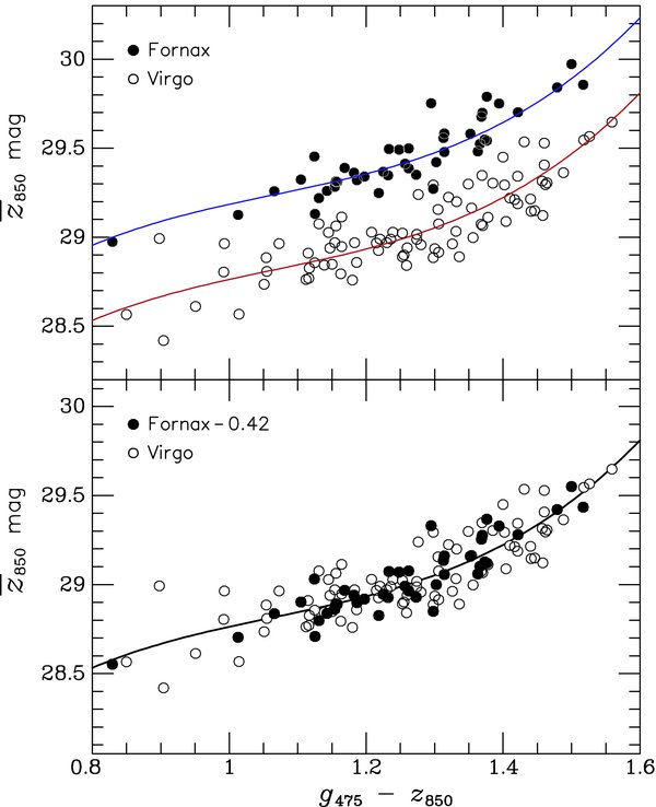
Figure taken from
Blakeslee et al., ApJ 694, 556 (2009)
The SBF method appears to give relatively precise distances when used properly; Blakeslee et al., ApJ 694, 556 (2009) claim an intrinsic scatter of only about 0.06 mag. We can check this by looking at a recent determination of the distances to galaxies in the Fornax cluster.
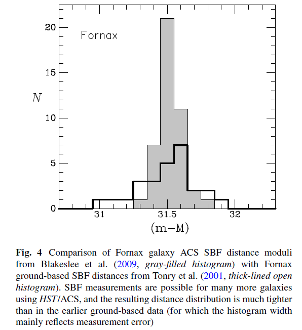
Figure 4 taken from
Blakeslee, J. P, ApSS 341, 179 (2012)
The technique has been applied to galaxies as far as about 20 Mpc, but there are hopes that it may be possible to use it for the Coma Cluster in the near future.
Copyright © Michael Richmond.
This work is licensed under a Creative Commons License.