 Copyright © Michael Richmond.
This work is licensed under a Creative Commons License.
When we measure some physical quantity experimentally, we usually incur some error in the measurement process, leading to an uncertainty in the result. Parallax is no exception: there are a number of sources of error in the measurement of very small angles between blobs of light from different stars. The topic for today is the sad, but true, fact that random errors in the measurements of parallax angles will NOT lead to "random" errors in the derived distances. We can expect to see a systematic error in distances measured via parallax.

I want to know the mass of each ball. My method:
Now, in step 2, reading the scale, I can't do a perfect job. My scale has markings for every 0.1 Newton, so I can't make readings any more precisely than that. However, my scale is well calibrated. I decide that there's an uncertainty of +/- 0.05 Newton in each measurement. Let's look at the results: both the mass I derive, based on my measurement, and the average ACTUAL mass of a large set of weights which give the same reading. I'll assume for the moment that g = 10 m/s^2 for simplicity. I'll also assume that the errors in measurement are uniformly distributed between -0.05 and +0.05 Newtons.
Ball    measured    derived   range of poss    range of poss    average
        weight (N)  mass(kg)   weight(N)         mass (kg)      mass (kg)
-------------------------------------------------------------------------
  A        5.20      0.520     5.15 - 5.25    0.515 - 0.525      0.520
  B        0.80      0.080     0.75 - 0.85    0.075 - 0.085      0.080
  C        2.10      0.210     2.05 - 2.15    0.205 - 0.215      0.210
  D        4.80      0.480     4.75 - 4.85    0.475 - 0.485      0.480
  E        1.20      0.120     1.15 - 1.25    0.115 - 0.125      0.120
-------------------------------------------------------------------------
Compare the mass I derive for each ball to the average mass of a whole bunch of similar balls which give identical readings. That is, in the first row, the "derived mass" column is my estimate of the mass of ball A: 0.520 kg. Now, if I find a box full of balls roughly the same size and shape as A, put them on the scale, and pick out all those which give a reading of "5.20 N", I'll have some which are just a bit more massive, and some just a bit less massive. If I weigh all these balls on a much more precise scale, and find their true masses, then average them all together ... I'll find the same value of 0.520 kg.
So there's no difference between a single calculated mass (0.520 kg) and the average value of a whole bunch of TRUE masses, all of which yield the same measurement (5.20 N). The difference is zero:
(average of true masses) - (mass derived from one reading) = 0
In other words, an error in the measurement of weight doesn't cause any bias in the derived calculation of mass.

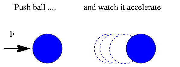
This time, however, I don't use a scale. Instead, I measure mass by pushing each ball gently with a standard force (10 Newtons), and measuring the balls subsequent acceleration:

My measured accelerations have an error of +/- 5.0 m/s^2, which I assume again to be uniformly distributed. Here are my measured accelerations, and the masses I derive from each one.
Ball    measured    derived   range of poss    range of poss    average
       accel(m/s^2) mass(kg)  accel(m/s^2)       mass (kg)      mass (kg)
-------------------------------------------------------------------------
  A       19.2       0.520     14.2 -  24.2    0.704 - 0.413      0.559
  B      125.0       0.080    120.0 - 130.0    0.083 - 0.077      0.080
  C       47.6       0.210     42.6 -  52.6    0.235 - 0.190      0.213
  D       20.8       0.480     15.8 -  25.8    0.633 - 0.388      0.510
  E       83.3       0.120     78.3 -  88.3    0.128 - 0.113      0.120
-------------------------------------------------------------------------
Compare the "derived mass" column in this table to the "average mass" column: they are NOT the same. The average of all possible masses which are consistent with the measured acceleration is LARGER than the mass derived from a single measurement.
(average of true masses) - (mass derived from one reading) >= 0
The size of this systematic bias depends on the mass of the ball. For very massive balls, the bias is large; for less massive balls, the bias is smaller. A very lightweight ball might have no perceptible bias at all.
  Q: Why does the size of the bias depend
        on the mass of the ball?
The root of the difference between the two examples above is in the connection between the measured quantity (which has some uncertainty in it) and the derived result. In the first case, we have:
mass = weight / g
In this direct linear relationship, an error of +10 0n weight leads to an error of +10 0n mass; and an error of -10 0n weight leads to an error of -10 0n mass. Symmetric errors in the measurement cause matching symmetric errors in the result.
But in the second case, the equation is
mass = F / accel
In this inverse linear relationship, an error in the positive direction does NOT have the same effect on the result as an error in the negative direction.
Well, let's qualify that claim just a bit: the errors in the result are actually pretty symmetric when the fractional error in the measurement is very small; it's only when the fractional error in the measurement becomes large that the asymmetric mistake in result becomes obvious. See for yourself.
Given a force of F = 10 N , and the relationship
mass = F / accel
  Measured       if wrong  yields   true accel true mass    error in
 accel (m/s^2)     by      (kg)      (m/s^2)     (kg)      result (kg)
----------------------------------------------------------------------
         10       0%        1.0       10.0        1.0          0.00

         10     + 1%        1.0        9.90       1.010     -  0.010
         10     - 1%        1.0       10.10       0.990     +  0.010

         10     + 5%        1.0        9.50       1.053     -  0.053
         10     - 5%        1.0       10.50       0.952     +  0.048

         10     +10%        1.0        9.00       1.111     -  0.111
         10     -10%        1.0       11.00       0.909     +  0.091

         10     +20%        1.0        8.00       1.250     -  0.250
         10     -20%        1.0       12.00       0.833     +  0.167

         10     +50%        1.0        5.00       2.000     -  1.000
         10     -50%        1.0       15.00       0.667     +  0.333
    ----------------------------------------------------------------------
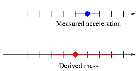
We can show this effect graphically: symmetric error bars on the measured acceleration lead to asymmetric error bars on the derived mass.

In general, an inverse relationship between measurement and derived quantity leads to asymmetric errors and a bias in the final result. That's not good. But in the particular case of parallax, there's an additional factor which accentuates the bias, making the problem even worse.
Space is big, really big, and it's full of stars. To a decent approximation, stars in the local neighborhood are scattered at random in all directions. Let's consider an "ideal" universe, which is full of identical stars, uniformly spaced at intervals of 1 parsec.
Suppose that we measure the parallax to one particular star, Abelix: π = 0.010 +/- 0.002 arcsec. Our best guess for the distance to Abelix is simply D = 1 / 0.010 = 100 pc. Fine. But now let's think carefully about the possibilities produced by the error in our measurement.
We can get a bit more quantitative. Exactly how many stars might turn out to have measured parallaxes within the range of 0.008 < π < 0.012 arcseconds? That corresponds to a range of distances from 125 pc < D < 83.3 pc.
         V  =  4/3 π [  (100 pc)^3  -  (83.3 pc)^3   ]

            ~  1,765,000   pc^3
which means that the total number of stars which might
APPEAR to have a parallax of 0.010 arcsec --
but are actually closer -- is about 1,765,000.
         V  =  4/3 π [  (125 pc)^3  -  (100 pc)^3   ]

            ~  3,992,000   pc^3
which means that the total number of stars which might
APPEAR to have a parallax of 0.010 arcsec
-- but are actually farther away -- is about 3,992,000.
There are more than twice the number of stars in the outer shell as in the inner shell. So, if we just pick one star at random which has a measured parallax of π = 0.010 +/- 0.002 arcsec, the chances are about 70 percent that the ACTUAL parallax is less than 0.010 arcsec, and the ACTUAL distance is larger than 100 pc.
In other words, when the uncertainty in a measured parallax becomes a significant fraction of the measurement itself, the chances are that the ACTUAL distance to the star is larger than the calculated distance. This effect was pointed out by Trumpler and Weaver in 1953 (and possibly by others even earlier), but received a very detailed treatment by Lutz and Kelker in 1973. It is now often called the Lutz-Kelker bias as a result.
  Q:  Hipparcos measurements have a typical
      uncertainty of +/- 0.001 arcsec.

      Estimate the bias in the distance
      to a star with measured parallax of
      0.005 arcsec.

      (Yes, to do this right involves an integral.
       If you want to make simple approximations
       in class, go ahead)
 Copyright © Michael Richmond.
This work is licensed under a Creative Commons License.