 Copyright © Michael Richmond.
This work is licensed under a Creative Commons License.
Copyright © Michael Richmond.
This work is licensed under a Creative Commons License.
Let's concentrate on the optical window, from about 4000 Angstroms to about 10000 Angstroms. Traditional astronomy deals with this narrow range of the electromagnetic spectrum because
There are other windows in the near-infrared (and at much longer wavelengths, in the radio), but one must use detectors which are not sensitive to visible light to record radiation at those IR wavelengths.
![]()
We can show the spectra of blackbodies with temperatures typical of ordinary stars (thousands of degrees Kelvin) in this optical region on a semi-logarithmic plot:
But it will be more useful to show the spectra in Flam on a linear scale. I have very roughly normalized the spectra so that their peak fluxes are nearly the same. The black box shows the "optical" portion of the spectrum.
Just how close to blackbodies are real stars?
It depends on which real star you pick.
If you choose a relatively cool star --
say, a K7 dwarf(*) -- a blackbody of the right
temperature is a pretty good model:
(*) don't worry, these terms will be defined in a later lecture
If, on the other hand, you examine the spectrum of a hot star, you will find that it differs very strongly from a blackbody in the near-UV:
What's the difference? As we'll discuss later in the course, the outermost portions of stellar atmospheres are largely hydrogen. In the red part of the optical, hydrogen is nearly transparent; thus, the blackbody-like radiation from the hot, dense gases below can fly out into space unimpeded. But in the blue part of the optical and the near-UV, hydrogen has many strong absorption lines.
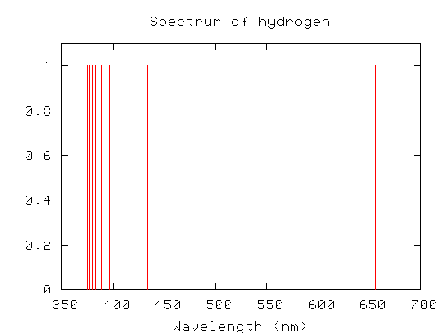
Photons with wavelengths below 3650 Angstroms will almost certainly be absorbed by a hydrogen atom as they pass through the stellar atmosphere, lifting the atom into an excited energy state. When the atom radiates away this energy, it usually does so by emitting a series of less-energetic photons at longer wavelengths. The strong absorption lines of hydrogen and other common elements act like a "blanket", preventing near-UV photons from escaping the star. This line-blanketing redistributes much of the ultraviolet energy of the star into the visible and infrared.
Astronomers figured out pretty quickly that it's nearly impossible to compare measurements made by different observers with different equipment and different detectors. Therefore, they defined a series of standard passbands, and tried to arrange their equipment so that it would always come close to one of these passbands. In real life, the passbands have been a function of all these factors
For simplicity's sake, we'll consider only the end result, and pretend that it is possible to reproduce a desired passband simply by choosing the appropriate filter. I'll use the words "filter" and "passband" interchangeably in the discussion which follows.
Optical passbands can be divided into three main groups:
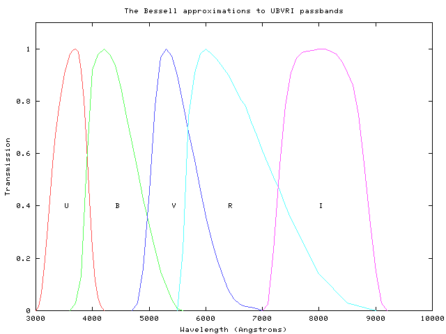
In 1990, Michael Bessell published a set of combinations of cheap optical glass filters which would reproduce reasonably well the classic Johnson-Cousins passbands.
The advantage of broadband filters is that they transmit lots of light; that means one can detect faint objects with short exposure times and small telescopes.
The transmission curves below are taken from the Kitt Peak filter set. I've normalized the curves so that the peak value is 1.0.
Although this set requires longer exposure times (or larger telescopes) to reach the same signal-to-noise as the wider filters, it has been carefully designed so that each filter samples a physically informative portion of a real star's spectrum. The u and v passbands, for example, lie just to the left and to the right of the strong break in the stellar spectrum (the "Balmer jump"); the ratio of the light gathered through these two passbands is a good diagnostic of stellar temperature.
I've normalized the curves so that the peak value is 1.0. Please note that very narrow filters don't follow any particular prescription: they are usually custom-made for some job. A set of on/off H-alpha filters at one observatory may not be the same as those at another observatory.
Narrow-band filters are usually designed in pairs, so that one includes a particular spectral line (in this case, the H-alpha feature), and the other includes only the continuum to one side of the line.

Suppose we settle on a passband -- the Johnson-Cousins V-band, for example. In order to figure out just how bright a star will appear when observed through this passband, we need to convolve the spectrum of the object with the transmission curve.
Note that the peak of the convolved spectrum lies to the blue of the filter transmission curve, because the stellar spectrum is "tilted" towards the blue.
The "area under the curve" of the convolution is related to the energy which should be measured by an instrument. This would be the correct quantity to compare to measurements if one had a device which really did record the incident energy. For example, one can make a bolometer out of a little chunk of metal painted black. Focus starlight on the metal; it will absorb all the energy and heat up. The amount by which its temperature rises is proportional to the energy which strikes it.
But most common optical detectors don't measure energy directly; instead, they count photons which strike the detector. Each photon which hits a CCD, for example, knocks free one electron. Thus,
           photon       photon     knocks free
        wavelength      energy   how many electrons?
        (Angstroms)     (ergs)
     ---------------------------------------------------
          4000         4.95 E-12          1

          6000         3.30 E-12          1

          8000         2.48 E-12          1
     ---------------------------------------------------
In other words, the output of the detector is NOT proportional to the amount of energy which hits it. In order to calculate properly the measurement from a photon-counting device, we need to
Over the relatively narrow range of the optical window, the difference between "energy detected" and "number of photons detected" can become considerable. If you are trying to predict a photometric measurement to an accuracy of a few percent, you must go through this complication.
Okay, suppose you do go through all these messy calculations. How do the resulting fluxes, or numbers of photons, correspond to magnitudes on the standard system? To a reasonable approximation, the magnitude scale is arranged in a conceptually simple manner: the star Vega
is defined to have magnitude zero in all passbands.
The real situation is a historical mess, and way too complicated for this course.
So, if we take the observed spectrum of Vega -- outside the Earth's atmosphere! -- and convolve it with the Johnson-Cousins passbands, we get the following energy flux and photon "flux":
   Passband      Energy Flux       Photon "flux"
               (erg/sq.cm/sec)   (photons/sq.cm/sec)
  ---------------------------------------------------
      U          2.96e-06            550,000
      B          5.27e-06          1,170,000
      V          3.16e-06            866,000
      R          3.39e-06          1,100,000
      I          1.68e-06            675,000
  ---------------------------------------------------
A simple number to remember for order-of-magnitude calculations is that a magnitude zero star will yield roughly one million photons per second per square cm through a broadband filter above the Earth's atmosphere.
Copyright © Michael Richmond.
This work is licensed under a Creative Commons License.