Simple Aperture Photometry by Hand

Aperture photometry is the measurement of light which falls inside a particular aperture; usually, we mean a circular aperture of some fixed size. The XVista tv command allows you to perform simple aperture photometry by pointing the cursor to a star and pressing the "a" key.

1. gathering the images for this exercise
2. selecting the right aperture
3. measuring instrumental magnitudes

Gathering the images for this exercise

The first thing you need to do is to gather a set of images to measure. I've chosen some images of the variable star IY UMa, taken on UT Apr 12, 2006, at the RIT Observatory. There are 100 cleaned images available, but you don't need them all. Please select a range of ten numbers between 1 and 100 -- say, 20 to 29. Then execute commands like the following to make copies of your ten images on the local machine.

  cp $dd/iyuma/iyuma-020.fit .
  cp $dd/iyuma/iyuma-021.fit .
     and so on 
  cp $dd/iyuma/iyuma-029.fit .

There's a faster way to copy these 10 files, using the Unix wildcard character '?' like so:

  cp $dd/iyuma/iyuma-02?.fit .

You should end up with ten cleaned images in your current directory, with names like iyuma-020.fit, etc. Try displaying one right now, just to make sure that nothing has gone wrong.

        tv iyuma-020.fit 

When you have all your images, look around at the students sitting near you. Help anyone who is having problems. We'll move on when everyone is ready.

Selecting the right aperture

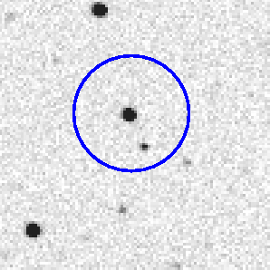
Before you can start measuring magnitudes, you need to pick a good size for the aperture. If you pick an aperture which is too big, you'll include light from neighboring stars:

The apertures below don't include light from neighboring stars ... but they are still large enough that MOST of the area included around a faint star is clearly background sky. The light from the star itself is concentrated at the very center.

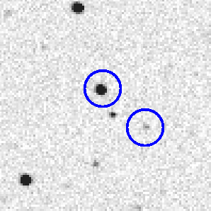
The goal is to pick an aperture which will include

• most of the light from the star but
• little extra light (and noise) from the background sky

A good compromise is an aperture which is a little bigger than the visible extent of faint stars:

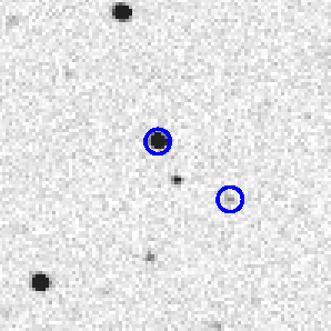
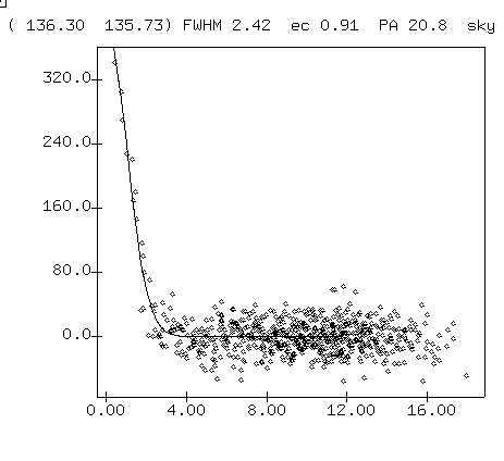
In practice, a good choice for the radius of an aperture is about 1.5 or 2.0 times the FWHM. You can quickly measure the FWHM by moving the cursor to an unsaturated star and pressing the "r" key. A little window showing the radial profile of the object should pop up, like this:

Exercises:

1. measure the FWHM of your images, in pixels
2. each pixel of these images is really a 3x3 binned "superpixel". The plate scale for these binned images is 1.85 arcseconds per pixel. What is the FWHM of your images in arcseconds?
3. calculate a good aperture size, in pixels
4. compare your aperture size to that of students using other sets of images. Are they all the same, or are there variations in the FWHM from set to set?

Measuring Instrumental Magnitudes

First, you need to set the size of the aperture. It is stored in the XVista symbol table, a little ASCII text file in the home directory of the CCD user. You can show the contents of the table by typing the XVista command xlet:

     xlet

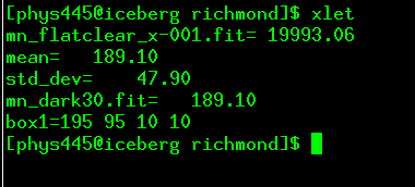
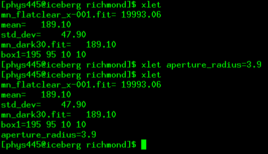
The aperture radius is controlled by the aperture_radius symbol; set it to the desired aperture radius in pixels:

     xlet aperture_radius=3.9

You also need to set the radii of the annulus used to measure local background sky values for each star.

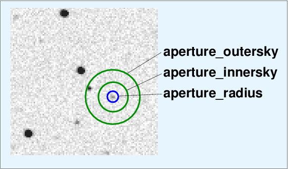
Reasonable values for the sky annuli are around 4-5 times the aperture radius for inner boundary, and around 6-7 times the aperture radius for outer boundary. It's okay if the annulus contains one or two stars, as long as the great majority of its pixels are purely background sky.

If you want to see just how big a radius of 10 pixels looks compared to the stars, you can define a circle at the position of a star (let's pretend it is at row 234, col 173) and then display it on all current images like so:

     circle 1 cr=234 cc=173 rad=10

     circle 1 show

Let's say you decide that the sky annulus should have radii 10 and 20 pixels.

     xlet aperture_innersky=10
     xlet aperture_outersky=20

Exercise: Determine an appropriate value for aperture_radius, aperture_innersky, aperture_outersky. We'll poll all the students and pick one set of values for everyone to use.

Now, once you've set the apertures, you are ready to measure instrumental magnitudes. Display a clean image with the tv command, move the cursor to a star of interest (sometimes it helps to use the "z" key to zoom in for a closeup), and press the "a" key.

The computer will print a line of values every time you press the "a" key.

1. row of stellar center
2. col of stellar center
3. total (counts - sky) in the aperture (counts)
4. number of pixels inside the aperture
5. instrumental magnitude of the object
6. background sky value inside the aperture (counts per pixel)
7. aperture radius (pixels)
8. inner sky annulus radius (pixels)
9. outer sky annulus radius (pixels)

The instrumental magnitude is NOT the same as the "standard magnitude" of the star that you would find in a catalog; instead, it is simply the total (counts - sky) value inside your aperture, converted into a logarithmic form like so:

         instrumental_mag  =  25.0  -  2.5*log10(counts - sky)

If you find that star A has an instrumental magnitude which is about 1.2 brighter than star B, then it is probably true that the catalog magnitude of A will be around 1.2 brighter than the catalog magnitude of star B. But the zeropoint of your instrumental magnitudes is arbitrary.

It sometimes helps to plot a radial profile with the "r" key. The graph will give you some idea for the signal-to-noise ratio (S/N) of the measurement.

The height of the peak of this radial profile is a measure of the (sky-subtracted) signal from the star. The scatter of the pixel values far from the center is a measure of the noise in the sky background. The ratio of the two is one way to estimate the S/N of the stellar measurement.

It's a pretty bad way to make an estimate, since it presumes that all the light from the star falls into a single pixel; but scientists often use this "peak-to-scatter" method for very faint signals, which may appear to have signal only in a central pixel or two.

                                            1
         percent uncertainty  =   100 * ( ------ )
                                           S/N

Exercise:

4. What is the S/N ratio, based on the radial profile above?
5. Estimate the precision of a single magnitude measurement of the star whose radial profile is shown above.

Watch out for bad images!

As you are analyzing a set of images, you may occasionally see something that doesn't look quite right. For example, my colleague Lew Cook was measuring the variable star OV Boo one night when he noticed this:

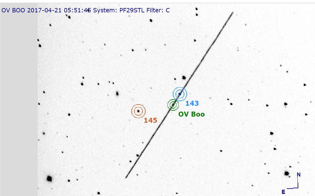
If you come across something that doesn't seem right, it's best to skip the image and leave it out of any further calculations.

Instrumental magnitudes of IY UMa and two comparison stars

Please measure by hand the instrumental magnitudes of the variable star IY UMa and two comparison stars in each of your images. Use the stars marked "A" and "B" in this chart:

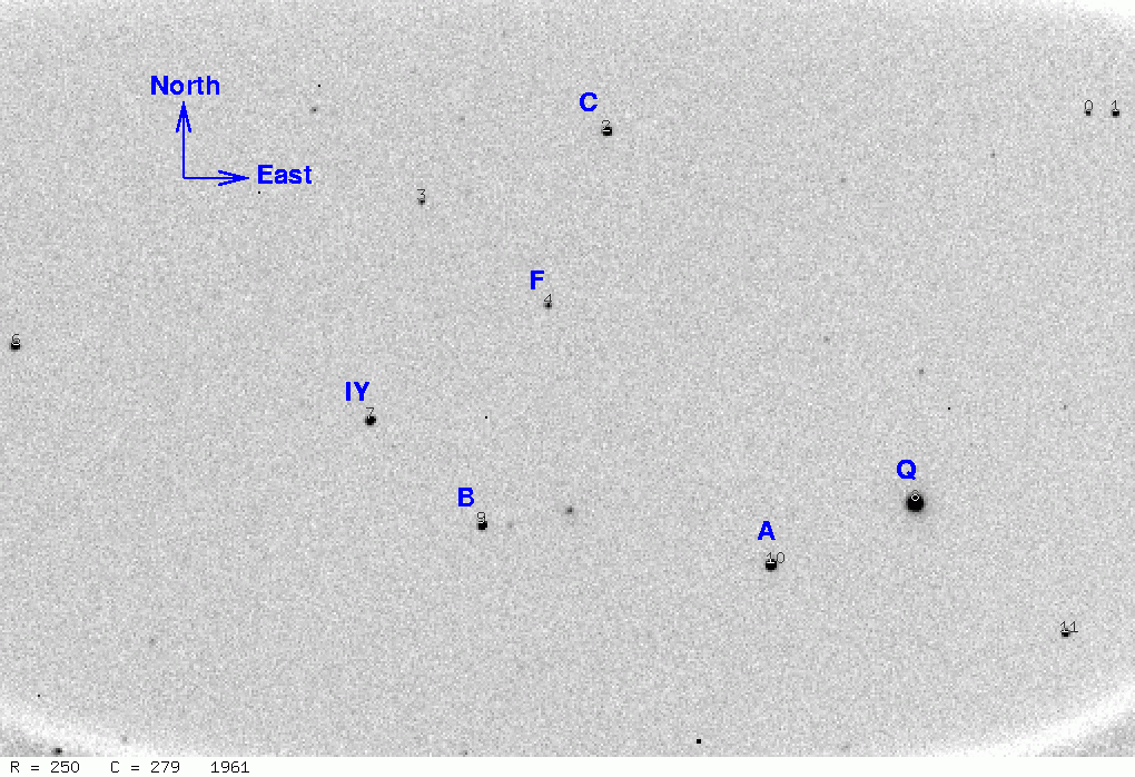
You should make a table which looks like this:

# image     IY       A       B       
1          13.079  12.592  13.670  
2          13.091  12.612  13.642  

After making your table, create a light curve -- a graph showing magnitude on the vertical axis (with bright at top, so smaller numbers at the top!) and time on the horizontal axis. Walk to the computer on which your instructor has created a simple spreadsheet. Type your numbers into the spreadsheet, making sure that your values go into the proper columns. After everyone has typed in his data, we will plot all the measurements.

Exercises:

6. Why didn't I ask you to use the brightest star in the field (marked "Q" in the chart) as a comparison?
7. Do you see any patterns in your light curve?

Differential photometry

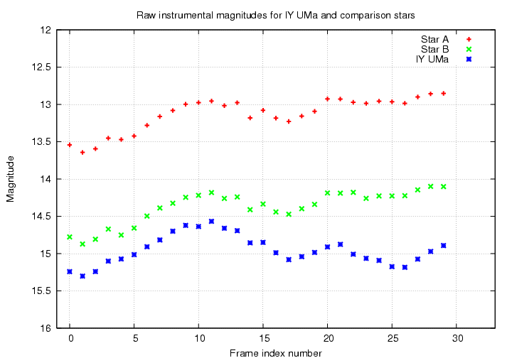
All the stars seem to grow brighter and fainter simultaneously.

Exercises:

8. What could cause these common features?

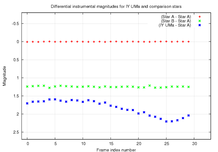
The cure for this symptom is to pick one star as a reference, and calculate the difference between this star and every other star in the field. For example, if you were to pick star "A" as a reference, you would calculate

         (IY - A)   (A - A)   (B - A)

For more information

• The RIT Observatory notes for UT Apr 12, 2006 provide more details on the fascinating variable star IY UMa.

Copyright © Michael Richmond. This work is licensed under a Creative Commons License.