 Copyright © Michael Richmond.
This work is licensed under a Creative Commons License.
Copyright © Michael Richmond.
This work is licensed under a Creative Commons License.
The methods we've discussed earlier are not as mathematically sound as trigonometric parallax, but they don't rely on THAT many assumptions.
Today's method requires pushing our assumptions a bit farther ...
When we try to apply the Globular Cluster Luminosity Function method, we will have to fall back upon a somewhat weak argument:
I don't quite understand how globular clusters form, or why they have a particular distribution of luminosities ... but I am going to ASSUME that the clusters around galaxy A have the same distribution as those around galaxy B
We will simple assume that if two groups of objects have a similar appearance, that their properties must be the same in detail. It's quite a step away from individual stars, for which we can work out the physics in detail, or even a population of many millions of stars. In the case of globular clusters, we may only detect a few tens or hundreds of clusters around any particular galaxy.
Okay, enough philosophy. Back to science.
Globular clusters are collections of 10,000 to 1,000,000 stars orbiting within a compact space of a few parsecs. The stars within them belong to very old populations; in some cases, it appears that they may date from the time of our Galaxy's formation, or even earlier.
When we look at globular clusters within our own Milky Way, we can see very clearly the individual stars (except when they get in each other's way near the center, perhaps).

Image of M80 courtesy of
NASA and
Wikipedia
The very nearest neighbors to our Milky Way, other members of our Local Group of Galaxies, host globular clusters which can just barely be resolved into groups of individual stars ... sort of. For example, in the Andromeda Galaxy, M31, consider one little region to the right of the center.

Image of M31 courtesy of
NASA, ESA, Benjamin F. Williams (UWashington), Zhuo Chen (UWashington), L. Clifton Johnson (Northwestern) and Joseph DePasquale (STScI)
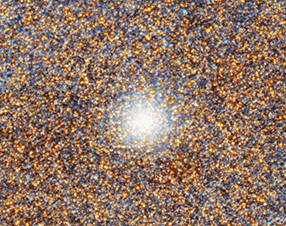
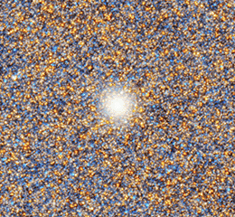
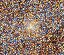
Images taken with the Hubble Space Telescope show globular clusters as clearly resolved clumps of stars. Can you find any in this region? There are at least four of them ...
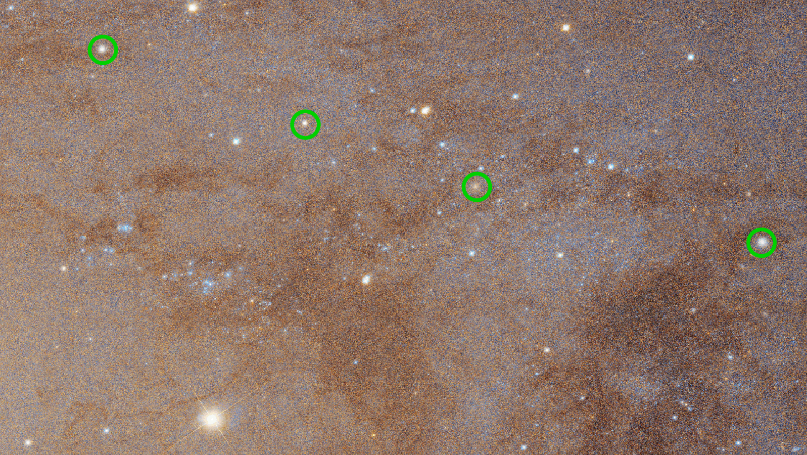
Here are closeups of each:

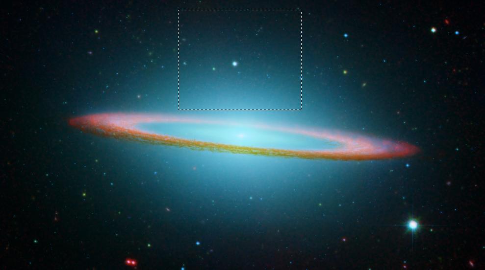
When we look at distant galaxies, we can't resolve the individual stars; instead, we just see a compact, bright ball of light. In this picture of the Sombrero Galaxy, for example, note the many, many little dots which appear blueish in color. (Click on the image below to enlarge)

Image of M104 from HST and Spitzer
courtesy of NASA/JPL-Caltech/University of Arizona
Here, I'll zoom in to show them more clearly.

Now, globular clusters are NOT identical: some are much larger than others, some are much more luminous than others. If we count the number of clusters in the Milky Way as a function of their absolute magnitudes, we find a roughly gaussian distribution. Yes, there's a tail at the low-luminosity end; no, for our purposes, that's not very important (why not?).
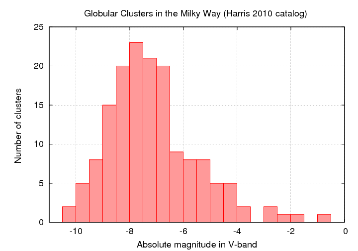
Figure based on data from
http://physwww.mcmaster.ca/~harris/mwgc.dat
   Q:  What is the ABSOLUTE magnitude of the peak of the
           luminosity function for globular clusters in the Milky Way?
If we look at the distribution of apparent magnitudes of globular clusters around other galaxies, we see something like a gaussian distribution (well, sometimes ... more on that in a moment). In the figure below, the left-hand panels show histograms of the GCs in a pair of Virgo Cluster galaxies.

Figure taken from
Jordan et al., ApJS 180, 54 (2009)
The right-hand panels in the figure above show a histogram of the COLORS of the GCs around those two Virgo galaxies. It seems that GCs come in two flavors, "red" and "blue"; the difference has something to do with metallicity. Is the mixture of flavors the same in all galaxies? Does it matter for the use of GCLF as a distance indicator? Good questions.
Villegas et al., ApJ 717, 603 (2010) compare the luminosity functions of globular clusters in two nearby clusters, Fornax and Virgo. Note the apparent difference in the width of these two distributions. Both distributions are thought to have the same intrinsic width, but because the Fornax cluster is a slightly more distant, incompleteness removes clusters from its faint end to a greater extent.
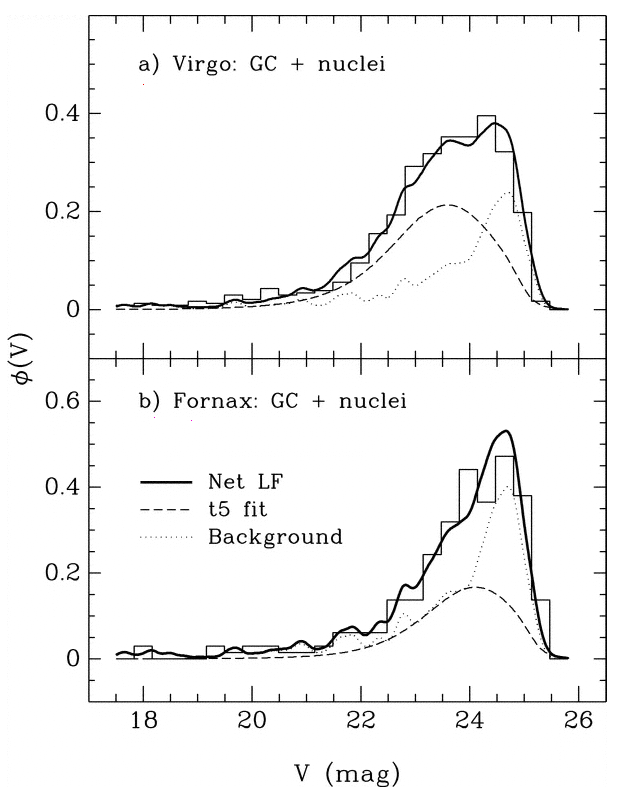
Figure taken from
Miller and Lotz, ApJ 670, 1074 (2007)
Let's put aside all these questions and just make the GIANT ASSUMPTION that the processes which formed globular clusters in the Milky Way also governed the formation of globular clusters around all other galaxies. In that case, the luminosity function for cluster around all galaxies should have the same absolute magnitude at its peak -- right? (Actually, in some cases, this might not be SO crazy -- see Harris et al., ApJ 797, 128 (2014))
  Q:  Choose either the Virgo or the Fornax
      distribution.  Compare it to the
      distribution of Milky Way GC absolute
      magnitudes.  Use it to estimate the
      distance to the Virgo or Fornax galaxy
      cluster.


            cluster        peak app mag     (m - M)        dist (Mpc)
  ------------------------------------------------------------------------
            Virgo

            Fornax

  ------------------------------------------------------------------------
This is a small digression from our discussion of the globular cluster luminosity function (GCLF) method of measuring distances.
Let's go back and take a closer look at that last graph. It showed histograms of the observed luminosity functions of GCs in the Virgo and Fornax clusters. Concentrate on the lower panel. Is the model of the luminosity function, shown in the long dashed line, really symmetric?

Figure taken from
Miller and Lotz, ApJ 670, 1074 (2007)
No. It isn't symmetric. There are more clusters on the "bright" side of the apparent peak, and fewer clusters on the "faint" side.
  Q:  Why should the observed histogram show
      more clusters on the bright side of the peak?
The answer is pretty simple: bright objects are easier to detect! If you are looking for stars or clusters or galaxies or just about any sort of object in an astronomical image, you generally have a better chance of finding the bright items than the fainter ones. Pretty obvious, really.
The trouble is -- this introduces a systematic bias, or selection effect, into any analysis based on the detected objects. Depending on the particular sort of analysis, this sort of selection effect might be insignificant, or it might be very important.
  Q:  In this case, we are matching the peak
      apparent magnitude of the GCLF in Fornax
      to the peak absolute magnitude of the
      GCLF in the Milky Way.

      If we do NOT take the selection effect
      into account, what will happen to the
      distance modulus we compute?
Let's consider a second example. Suppose that we are interested in open star clusters, and we are making a catalog which contains the size of each cluster. We take a picture of the cluster Perseus 3 and see the pattern of stars below. The scale bar is marked in arcseconds.
Q: What is the radius of the cluster?
A few years later, another astronomer is granted time on a bigger telescope and takes a series of exposures of Perseus 3 with a range of exposure times. Click on the picture above to see the results of his work.
Q: What is the radius of the cluster?
So, how can we deal with this menace to quantitative measurements? We must counter-attack with a quantitative correction for the effects of the varying degree of completeness. What we need is a way to describe the probability that an object is detected as a function of its magnitude. Not as simple as
but more sophisticated, like this:
If someone else has studied this particular region of the sky with a bigger telescope some time in the past, and published a detailed catalog of the objects in the area, then we can compare that catalog to the objects in our study to make this sort of table.
Alas, in most cases, there is no pre-existing deep catalog of objects in the area which one is examining.
  Q:  How can we make any accurate statements
      about the probability of detection if don't
      really know what we ought to be seeing?
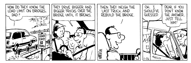
In the "old days", this was a tough problem. Since we have these newfangled devices called computers, however, there is a straightforward procedure we can follow to get a good, quantitative measure of incompleteness. The following Calvin and Hobbes comic strip may give you a clue ...
Start with some image showing the region of interest. This is a portion of the XMM-Newton/Subaru Deep Field.
Use some tool to find and measure the properties of all the objects in the image.
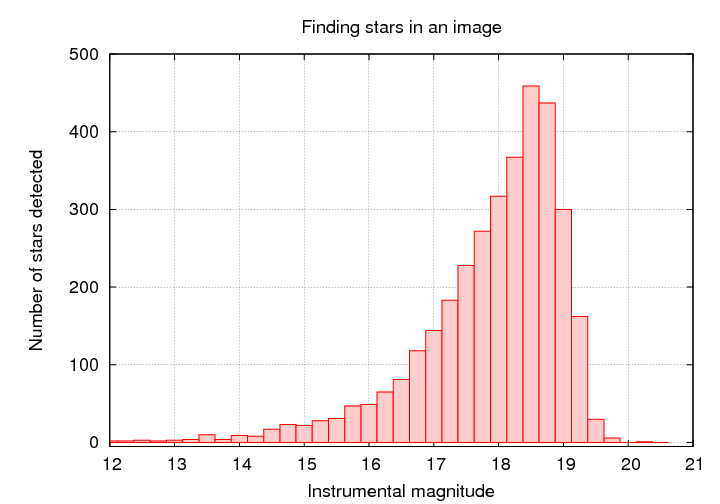
   Q:  At what magnitude do you think
       we fail to detect stars?
Now, the tricky part: use some tool to generate a set of fake objects, with the same size and shape as real objects, at random locations. Add those fake objects to the original image.
It's pretty easy to see the fake stars in the image above, isn't it? Try an image with fainter fake stars ...
Run this synthetic image, with real and fake objects, through your object-finding tool. Compare the list of objects found to the list of fake stars added. Compute the fraction of all the fake objects which were actually detected by your software.
Repeat for fake objects covering a wide range of magnitudes.
You can then make quantitative statements about the fraction of REAL objects which were (probably) detected by your software.
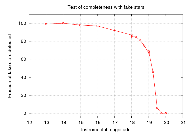
The point at which the fraction of objects detected falls to 50% is commonly used to define the completeness limit or plate limit. You must be very, very careful if you attempt to use measurements which are close to, or -- heavens above! -- beyond the completeness limit.
Fleming et al., AJ 109, 1044 provides a nice little analytic function which may work well to model the fraction of objects detected as a function of magnitude.
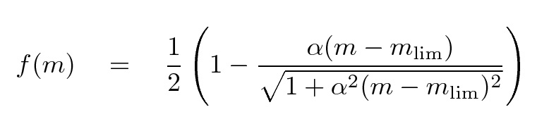
That function makes a gentle "sigmoid-ish" transition from 1.0 to 0.0 over a range which can be adjusted by the parameter α. It's similar to the shape seen in, for example, the case of stars in the XMM-Subaru Deep Survey.
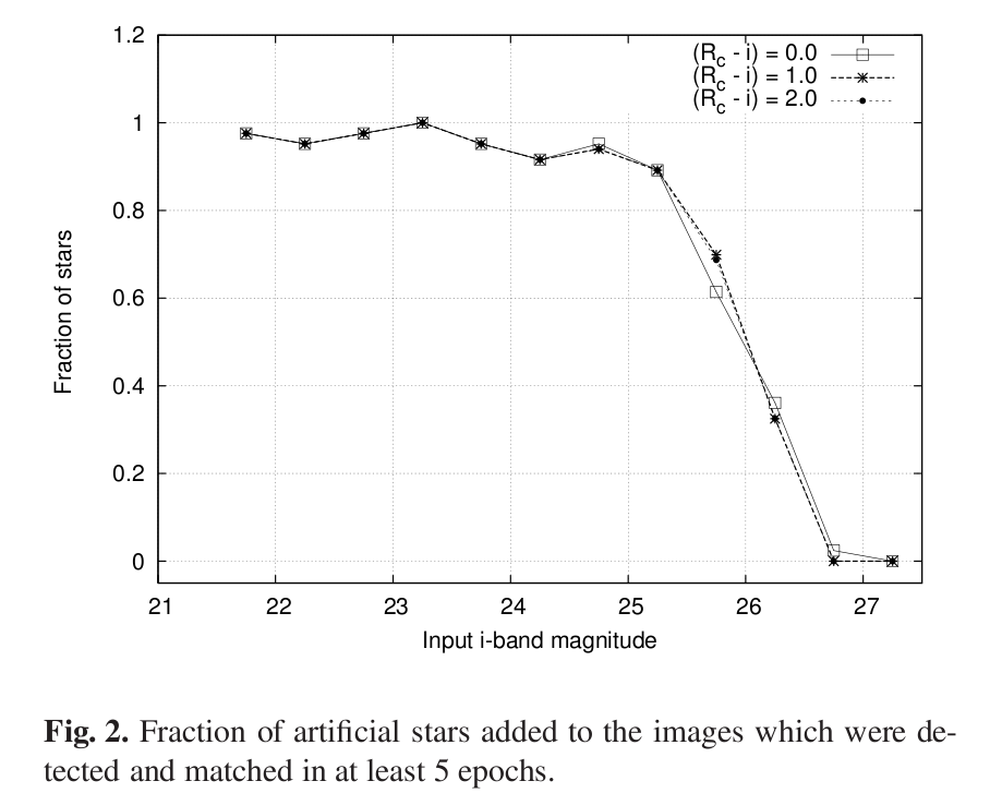
Figure taken from
Richmond et al., PASJ 62, 91 (2010)
The GCLF method came back into the news in 2017 when astronomers all over the world focused their telescopes on a distant galaxy called NGC 4993. On Aug 17, 2017, the LIGO and Virgo gravitational wave telescopes detected a burst of radiation which was eventually narrowed down to the outskirts of this elliptical galaxy.
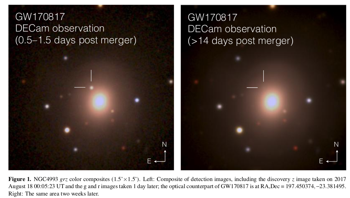
Figure 1 taken from
Soares-Santos et al., ApJ 848, L16 (2017)
It turned out that this was no ordinary merger of two black holes; instead, this was the first (and one of the very few to date) mergers of two neutron stars to be discovered via gravitational waves. Because the merger of neutron stars is predicted to produce a large amount of electromagnetic waves, in addition to gravitational waves, this galaxy quickly became one of the best-studied objects in the sky.
But how far away was it?
A team of astronomers at Seoul National University took up the challenge. They identified a set of Hubble Space Telescope images of this galaxy through the F606W filter, which is a bit redder than the standard V-band filter -- but not too different. If they could identify globular clusters surrounding this galaxy, then perhaps they could estimate its distance. In the figure below, the HST image is shown in the right-hand panel; the inset bordered in red is a zoomed-in view of the image after a model of the galaxy's light has been subtracted.
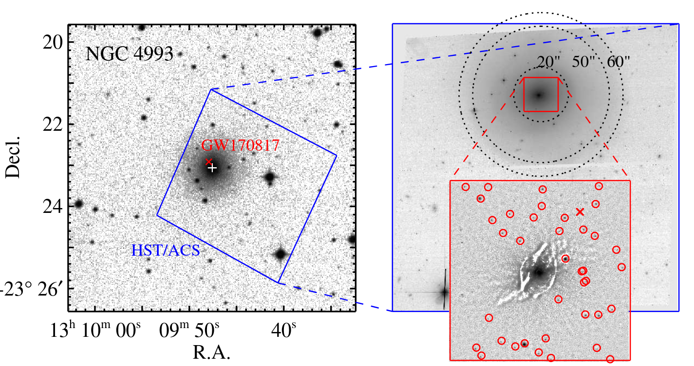
Figure 1 taken from
Lee, Kang & Im, ApJ, 859, 6 (2018)
The authors identified many faint little point sources around the galaxy -- but were these really globular clusters, or just background galaxies?
   Q:  How might we distinguish globular clusters belonging to
          NGC 4993 from random background objects?
One way is to examine the spatial location of the candidates. Real globular clusters should be concentrated near the host galaxy, while background objects ought to appear everywhere with a uniform distribution. And, indeed, certain candidates WERE concentrated around NGC 4993:

Figure 4 taken from
Lee, Kang & Im, ApJ, 859, 6 (2018)
After making corrections for these contaminating background galaxies, Lee et al. were able to graph the distribution of globular clusters around NGC 4993.

Figure 5 taken (and a bit modified) from
Lee, Kang & Im, ApJ, 859, 6 (2018)
  Q:  What is the apparent magnitude of the peak of the globular
            cluster luminosity function?


  Q:  Assuming that the absolute magnitude is MV = -7.9,
            what is the distance modulus to this galaxy?
The globular cluster technique may be losing some popularity now, but it was one the popular methods for nearby galaxies in the past because ground-based telescopes could measure the properties of globular clusters out to large distances. With HST, it can be used out to Coma and beyond.
Copyright © Michael Richmond.
This work is licensed under a Creative Commons License.