 Copyright © Michael Richmond.
This work is licensed under a Creative Commons License.
Copyright © Michael Richmond.
This work is licensed under a Creative Commons License.
Now that we've seen pictures of the cosmic microwave background (CMB), we can start to ask some questions about it. Today, we'll focus on two in particular: WHY is there a CMB (what created it?), and how can astronomers make use of all those little spots in the CMB maps made by COBE and other satellites?
In order to explain all those microwaves flooding the sky from all directions -- in a very uniform way -- we need to spend some time on one particular theory of the origin of the entire universe: the "Big Bang" theory. In the 1940s, astronomers and physicists had not yet settled on even the rough outlines of the universe's history. At that time, two of the most widely accepted ideas were
In a radio interview in 1949, the English astronomer Fred Hoyle, a proponent of the steady-state theory, used the following words to describe the competing idea.
Text taken from
Fred Hoyle: An Online Exhibition ,
courtesy of University of Cambridge
It actually took quite some time for other astronomers to adopt the phrase "Big Bang" for this theory; as Helen Kragh shows, technical papers didn't use it frequently until the 1970s.
What is the Big Bang Theory? There are many good explanations in books and on-line, but for our purposes of understanding the CMB, we can simplify it greatly into the following short story. You might look at the left-hand side of the picture below as we go over these stages. Note that all the times I've listed are only approximate.
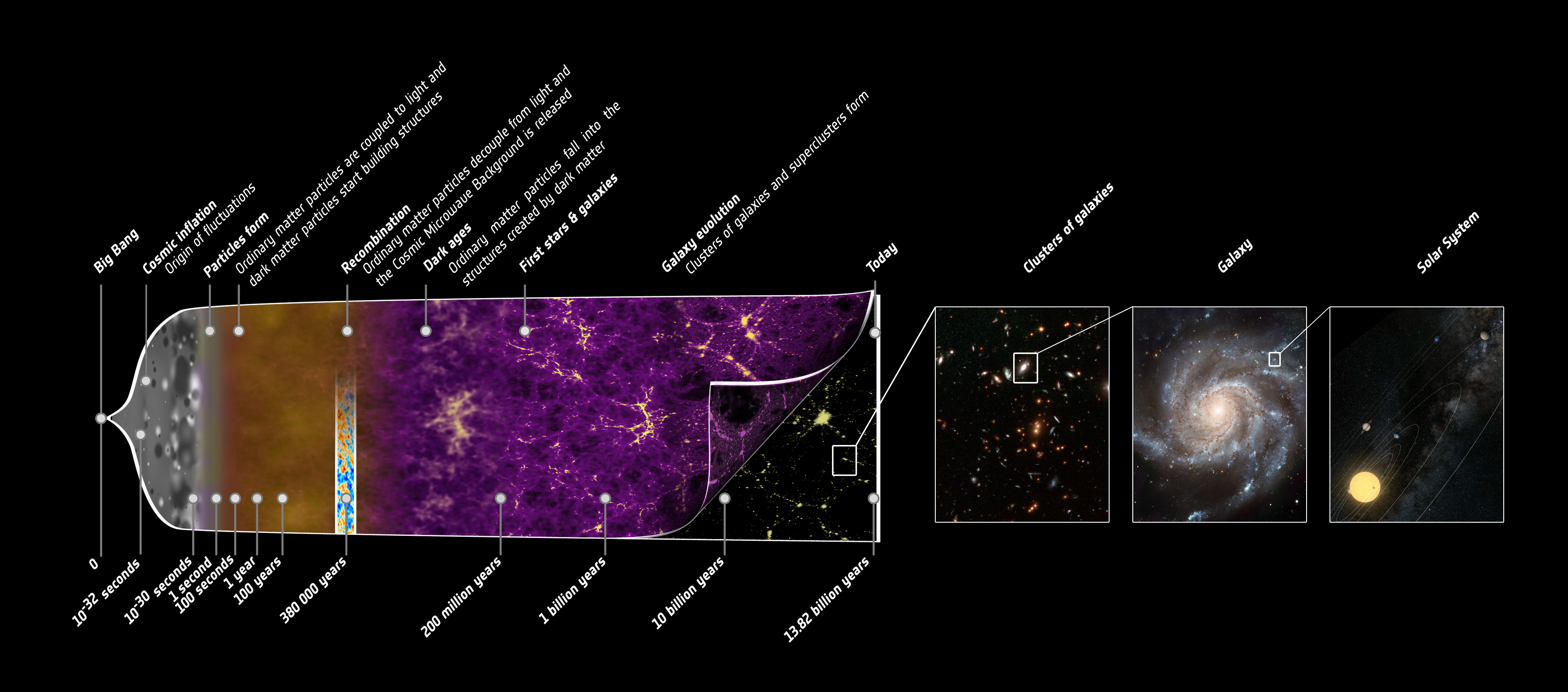
Image courtesy of
NASA
protons, electrons, neutrons, photons
Let's pause here, at 20 minutes after the Big Bang, to take a slight detour on our way to explain the CMB. The nuclei of chemical elements have just been formed, and their relative numbers will remain (mostly) unchanged over the next few billion years. Can we learn anything about the conditions in the early universe from the present-day mixture of chemical elements?
In a way, the early universe is like a gigantic test kitchen, in which an enormous dish of food is being prepared. In real life, the result of the cooking process depends crucially on how long one keeps the material on the heat.
The same is true of the primordial soup. At temperatures below T = 109 Kelvin, the protons and neutrons can fuse to form simple atomic nuclei. The longer the simmering -- and the denser the material during the simmering period -- the more fusing takes place. The nuclei which can form during this "nucleosynthesis" are
By far the most common reaction is for protons and light nuclei to combine to form Helium-4, the ordinary form of helium. The denser the soup, and the longer it simmers within the appropriate range of temperature, the more hydrogen is turned into helium. The relative amount of the other products -- deuterium, helium-3 and lithium-7 -- also depends on density and duration.
The energies of particles during this "simmering" phase of the universe are between 0.1 MeV and 1.0 MeV, which can easily be reproduced in terrestrial laboratories. Physicists have measured very accurately the rates at which all the various reactions between these particles and nuclei take place, and can make confident predictions for the relative amounts of each product after any particular duration of time. One can put all the information into a single picture:
To read this graph, pick some particular combination of density and duration (denoted by the symbols Ωbh2) along the bottom axis; then, draw a vertical line at that position. Where the line crosses each element's pathway is the predicted relative abundance of that element.
For example, in a low-density universe, we ought to find

But that's just an example. What are the ACTUAL ratios of these light elements that we observe in the real universe? A recent review article from 2014 provides the following summary. The yellow boxes show the range of elemental abundances that we observe.
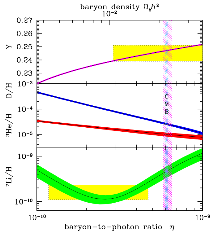
The helium and deuterium values agree and imply that the ratio of baryons to photons was around 6 x 10⁻¹⁰, and that the value of baryon density is around 0.02 = 2 percent of the critical value. However, the abundance of lithium seems much lower than expected. Astronomers think that some of the primordial lithium in the universe may be destroyed inside stars, but this is still an area of active research.
Okay, time to return to the expanding universe. When we left, it was t = 20 minutes after the Big Bang. What happens next?
Now, at this point, the universe is filled with a very hot (hundreds of millions of degrees) and very dense plasma, in which atomic nuclei, free electrons, and high-energy photons fly at very high speed and collide violently. The density is so high that the photons constantly smash into other particles before they can travel very far; the mean free path of the photons is tiny. In other words, the photons are trapped within their local collection of particles, and are unable to move over large distances.
The universe continues to expand and cool, expand and cool, and the density of material continues to decrease. A long time passes -- hundreds of thousands of years! -- with very little other change.
This transition, when the material filling the universe changed from an IONIZED plasma to a NEUTRAL gas, is the key event in forming the cosmic microwave background.
Photons react very differently with CHARGED particles than they do with NEUTRAL atoms. In very simple terms, charged particles have a large cross-section for interaction with photons. That means that a photon can't fly freely through an ionized plasma: due to the frequent collisions, the photon just keeps bouncing around in circles. In other words, a plasma is opaque, and keeps photons trapped within small regions.

On the other hand, the cross-section between photons and neutral atoms is (in general) much smaller. If a photon encounters a neutral atom, there is a very good chance that it may pass through it and continue moving on its original path. In other words, neutral gas is transparent, allowing photons to fly freely through it.
![]()
Okay, back to the very young universe. As long as the temperature was high enough to keep electrons from combining with nuclei, the photons were trapped together with the surrounding matter. If there was a slightly denser clump of gas, then the photons in that region were also clumped together, and could not escape to other regions of space. As strange as it may sound, at these very early times, the PHOTON DENSITY had small variations, too, exactly following the variations in the density of matter.
But when the temperature dropped low enough for the electrons to combine with nuclei and form atoms -- all of a sudden, the photons were able to escape and fly off into space in all directions. We call this drastic change decoupling, because matter and photons were no longer tied together strongly. At this point, a small clump of matter could collapse due to gravitational forces, but photons in the area could simply pass through it. The density of matter and photons no longer followed each other.
Now, imagine that we are floating in space just a short time after decoupling has occurred. We see photons coming from all directions, produced by hot, dense gas at a temperature of about T = 3000 Kelvin.
  Q:  What sort of spectrum does a very dense, hot gas produce?


  Q:  If the gas has a temperature of T = 3000 Kelvin, what is the
          wavelength at which the spectrum reaches its peak?
Suppose that when we look to the right, we see a region of space which was slightly more dense and hot than the average. That means that when the photons escaped from that region, their spectrum was that of a blackbody with a slightly higher temperature, and so the peak of their spectrum lies at slightly shorter wavelengths.
On the other hand, suppose the region to our left was one with a slightly lower density and temperature of gas. The photons which escape from this area have a spectrum with a slightly longer peak wavelength.
In summary, when photons decouple from the gas at this moment, their spectrum preserves a signature of the density and temperature of the gas from which they radiate. Because the universe is now transparent, those photons are free to fly through space for billions and billions and billions of years, unchanged, until they run into our telescopes and show us a picture of the variations in gas temperature at that long-ago moment when electrons combined with nuclei.
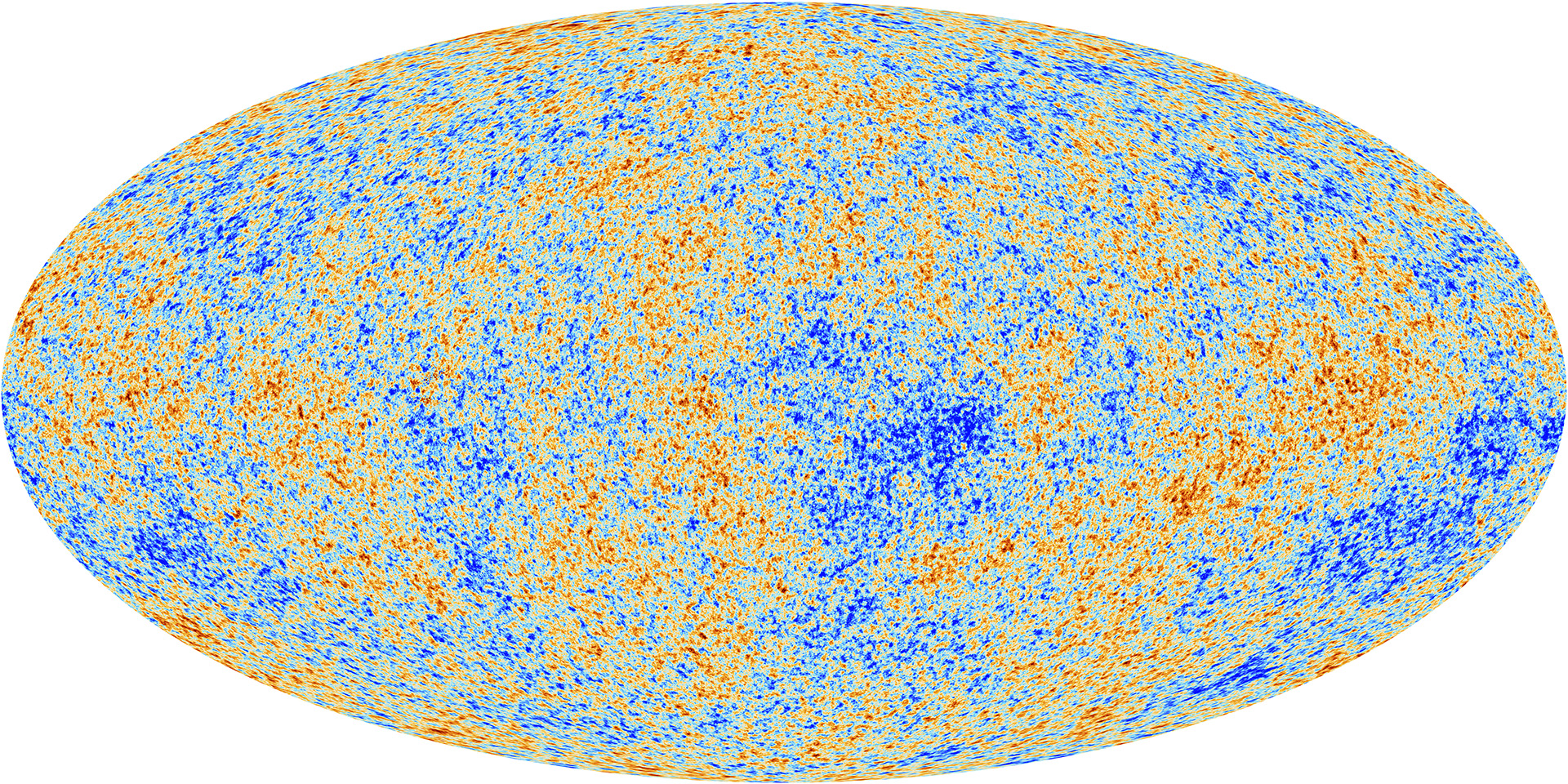
Image courtesy of
ESA and the Planck Collaboration
And that's what we see -- a map of the gas density and temperature in the early, early universe.
Hey -- wait a minute. When the photons were emitted by the hot gas, at T = 3000 K, the peak of the spectrum was around 966 nm, in the near-infrared portion of the spectrum. But we've been talking about the Cosmic MICROWAVE background, not the Cosmic Infrared Background.
   Q:  What happened to the photons between t = 300,000 years after
            the Big Bang (when they were created),
            and t = 13.7 billion years after the Big Bang (when
            we observed them)?
Right. Over those billions and billions of years, as the universe expanded, the photons were str-e-e-e-tched out by the expansion of space. Remember the scale factor a(t), which keeps track of the changes in the size of the universe? If a(t) increases, then the wavelength of photons increases by the same amount.
The peak of the CMB we observe now is around 1.06 mm, much longer than the original peak. This ratio of the observed wavelength to the emitted wavelength can be used to define a useful quantity called redshift.
Q: What is the redshift of the photons which make up the CMB?
Hey -- you got the same answer as the people who made this diagram!
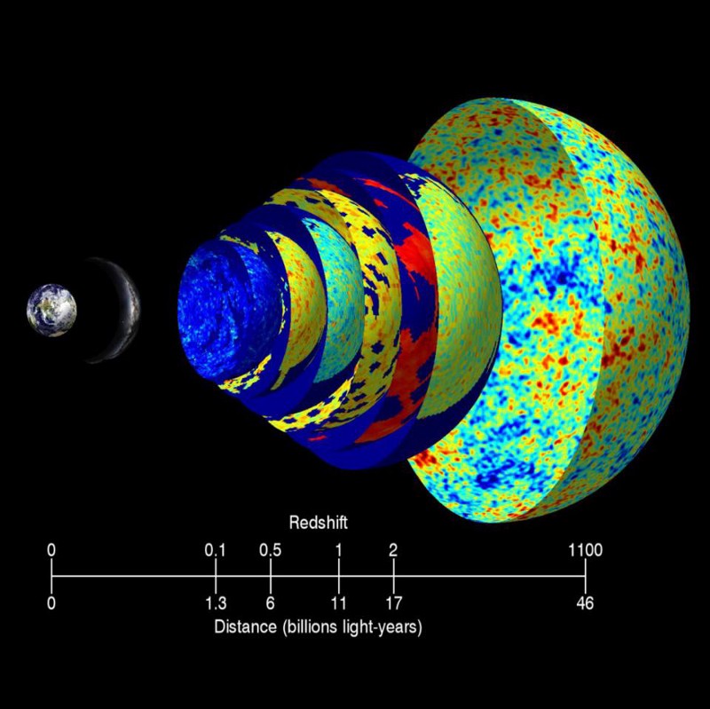
Image courtesy of
Earth: NASA/BlueEarth; Milky Way: ESO/S. Brunier; CMB: NASA/WMAP
The diagram below is somewhat out of date, as it doesn't take into account the most recent JWST results, but it might give you an idea for how much FARTHER AWAY the cosmic microwave background is than any ordinary stars or galaxies that we can see.
(Hint: the scale on the x-axis is NOT linear; just pay attention to the numbers)
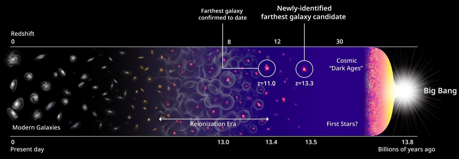
Image courtesy of
Harikane et al., NASA, EST and P. Oesch/Yale
  Q:  What is the largest redshift value for any galaxy we have
            measured so far?


  Q:  How does that compare to the redshift of the CMB?
It may look like a random assortment of small blobs, but the CMB actually contains a wealth of information about the properties of the universe at the time it was formed; one just has to look at it in the appropriate manner, or with the proper tools.
Let's start with a very simple approach: what's the typical size of the blobs? Well, one could try to look at one of the all-sky maps, like the one from Planck below. Let's see -- the equator should wrap all the way around the sky, an angular distance of 360 degrees. Could we just count the blotches across the middle of the picture?
Image courtesy of
ESA and the Planck Collaboration
Perhaps it would be easier to focus on a small region of the sky. The section below is a portion of a map made by the ground-based ACT. The grid marks around the edges of the image are separated by 2 degrees.
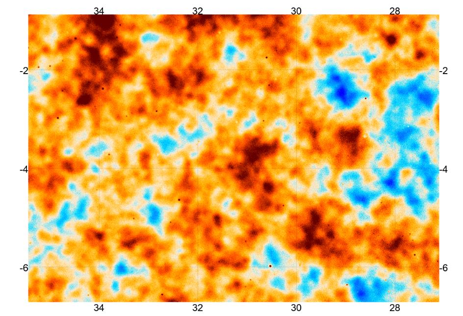
Image taken from
Mallaby-Kay et al., ApJS 255, 11 (2021)
Q: What is the typical size of a blotch in the CMB?
Okay, that's one way of analyzing CMB maps. It's easy to understand, and easy to carry out, but it yields just one number: the typical size of an individual hot or cold region.
There are more sophisticated techniques for finding numbers in these maps; they are harded to understand, and take more work, but they give us a LOT of extra quantitative information. We can then compare all those numbers against the predictions from various models of the evolution of material in the universe, and so test models versus observations.
One of these more sophisticated techniques is called the two point correlation function. The basic idea can be explained reasonably succinctly.
Given a random CMB spot in a location, the correlation function describes the probability that another spot will be found within a given distance.
A paraphrase from from Peebles, "Principles of Physical Cosmology" (1993)
How can one measure this probability of finding another spot at some given distance away from a given spot? Well, one method is to start with a map of spots, divide them up in pairs -- all possible pairs! -- and measure the distances between them. The number of pairs with any given separation is a measure of the probability that one will find a second spot at that distance from a first spot.
It's a lot easier to understand if you just watch someone do it. Click on the picture below to start a brief animation.
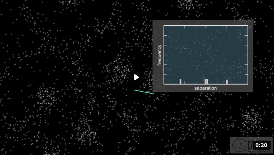
Image and animation courtesy of
Wikimedia and Arc Centre of Excellence for All-Sky Astrophysics
What can we learn from this two-point correlation function? It turns out that we can learn a LOT about conditions in the early universe ... but that will have to wait for next time.
Copyright © Michael Richmond.
This work is licensed under a Creative Commons License.