 Copyright © Michael Richmond.
This work is licensed under a Creative Commons License.
Copyright © Michael Richmond.
This work is licensed under a Creative Commons License.
A photon created within an optically thick medium will be scattered or absorbed and re-emitted many times before it finally escapes. How many times? And how long will it take to escape? We can't provide an exact answer for any particular photon, but we can make a decent estimate in a statistical sense of the average number of steps required, by using random walk analysis.
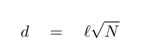
The basic idea is simple: given a mean free path ℓ (that's "the letter ell", not a numeral one), and a random distribution of scattering angles, determine the overall displacement d of the photon after a certain number N scattering events.

Let's follow this photon for a while. The picture above shows its progress after N=5 steps. How about N=10 ...

or N=15 ....

It turns out that the statistical average of the overall displacement d after N steps is simply
The total distance covered by the photon during this journey will of course be simply N * ℓ. If you know the speed of the photon -- and you do! -- then you can figure out the time it takes for the photon to make the trip.
Energy is generated at the center of the Sun by reactions in which hydrogen nuclei fuse together to form helium. These reactions release both energy, in the form of gamma ray photons and kinetic energy of the particles involved, and neutrinos.
Almost all of the neutrinos fly straight out of the Sun, not interacting at all with any of the atoms in the core, the intermediate layers, or the outer atmosphere of the Sun. Neutrinos are wierd that way. For our purposes, we can say that they travel at the speed of light. Physicists at several labs around the world operate "neutrino telescopes" that detect these neutrinos coming from the Sun.
Photons, on the other hand, do interact with atoms and ions and electrons. The path of a photon from the center of the Sun to the photosphere is a very complicated one, full of twists and turns and backtracking. Detecting photons from the outer atmosphere of the Sun is simple, of course: just look up!
Suppose that the Wicked Witch of the West waves her magic wand and turns off all fusion reactions at the center of the Sun.
Yes, yes, there would be dramatic events due to gravitational forces pulling the core in on itself ... ignore them for now.
  Q:  How long does it take a neutrino to travel from the core of
           the Sun to the Earth?


  Q:  How quickly will neutrino telescopes notice that something
           has changed?
  Q:  How long does it take a photon to travel from the core of
           the Sun to the Earth?

           For simplicity, assume that the mean free path of a photon
           EVERYWHERE in the solar interior is the same as the mean
           free path in the photosphere, which we estimated earlier
           to be 0.2 mm.


  Q:  How quickly will ordinary people, walking around outside,
           notice that something has changed?
The assumption that the mean free path of a photon in the photosphere is the same as the mean free path in the inner regions of the Sun is a poor one. The density of material increases greatly toward the center, which means that the mean free path will decrease. Our estimate above was a LOWER bound to the time it would take a photon to travel from core to photosphere; in one of this week's homework problems, you will compute the mean free path of a photon in the solar core and use that to estimate an UPPER bound to this time.
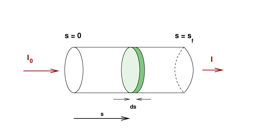
What happens when a beam of light of specific intensity I0 encounters a slab of some material? As we saw last time, if the material has some opacity, some of the light will be scattered or absorbed, and so the intensity leaving the slab will be smaller than the original intensity. For simplicity, let's assume that the material has some uniform density ρ and opacity κ.
In the diagram below, I've drawn the slab as a cylinder, which helps me to visualize the situation. If we use the variable s to denote location within the cylinder, along the path of the light beam, then we need to figure out the effect of the material as the beam travels from s = 0 to s = sf.

It helps to consider one very thin "slice" of the material, located at some distance s from the left end, and of thickness ds.
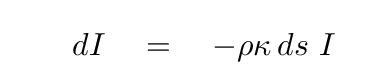
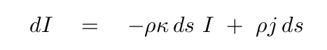
As light travels through this little slice, its change in intensity depends on the incoming intensity, the density, the opacity, and the thickness of the slice:
If we re-arrange terms a bit, and then define the optical depth τ = ρ κ s
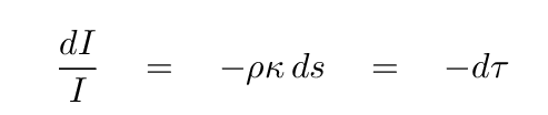
then it's easy to integrate both sides. We find that the intensity falls exponentially as the beam travels a distance s through the cylinder -- or, equivalently, through an optical depth τ = ρκs.

![]()
But what if the material in this cylinder is more interesting? What if, in addition to interacting with the incident light coming from the left, this material can also interact with photons from regions above or below the cylinder? Some of those photons might bump into atoms in the little slice and bounce off in exactly the right direction (to the right) to join the incoming beam. In short, what if this material acted as a SOURCE of light and not just a sink?
How much light would be produced within a tiny slice of length ds? This SOURCE of light would depend upon the amount of material inside the slice, so density ρ would come into play; but it should not depend on the intensity of the incoming light. We'll use a new letter, j, to describe the emissivity coefficient of the material: the amount of light it produces per unit of stuff. Most important of all, this term will produce an INCREASE in the light, so it must have a positive sign. So, we could write the change in intensity as the light traverses the tiny little slice as
If we divide both sides of this equation by density, opacity, and the little length ds, we get

In that final step, we have defined a quantity S known as the source function. Note that this source function has the same units as specific intensity: power per area per wavelength per steradian. In MKS-like units, watts per square meter per Angstrom per steradian.
Let's go back to the schematic diagram of light travelling through a cylinder of material. Our new equation -- the equation of radiative transfer, or simply "the transfer equation" -- tells us how the intensity of light changes as it goes through the teeny slice of width ds. The result will depend on the relative sizes of I and S.
If I > S, the amount of light scattered OUT of the beam is larger than that scattered IN from the surroundings. In that case, the light will grow a bit dimmer.
On the other hand, if I < S, then the amount of light scattered IN is larger, and the intensity of the beam will be slightly larger when it leaves the little slice.
There's one other interesting case. Suppose that this cylinder lies within a big box of gas which is in thermodynamic equilibrium. In that case,
What sort of behavior can we expect as a result of radiative transfer? Let's pick a very simple situation: a material with constant density and composition everywhere, so ρ and κ are both constant, AND a constant source function S as well. If we send a beam of initial specific intensity I0 into such a region, what will happen to it?
To find out, we integrate the radiative transfer equation with respect to position s, which yields
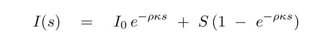
What does this mean for our beam of light? As it moves through the material, the initial intensity is gradually extinguished, and the source function becomes increasingly responsible for producing photons. After the beam has travelled several optical depths into the material, its intensity approaches the source function.
![]()
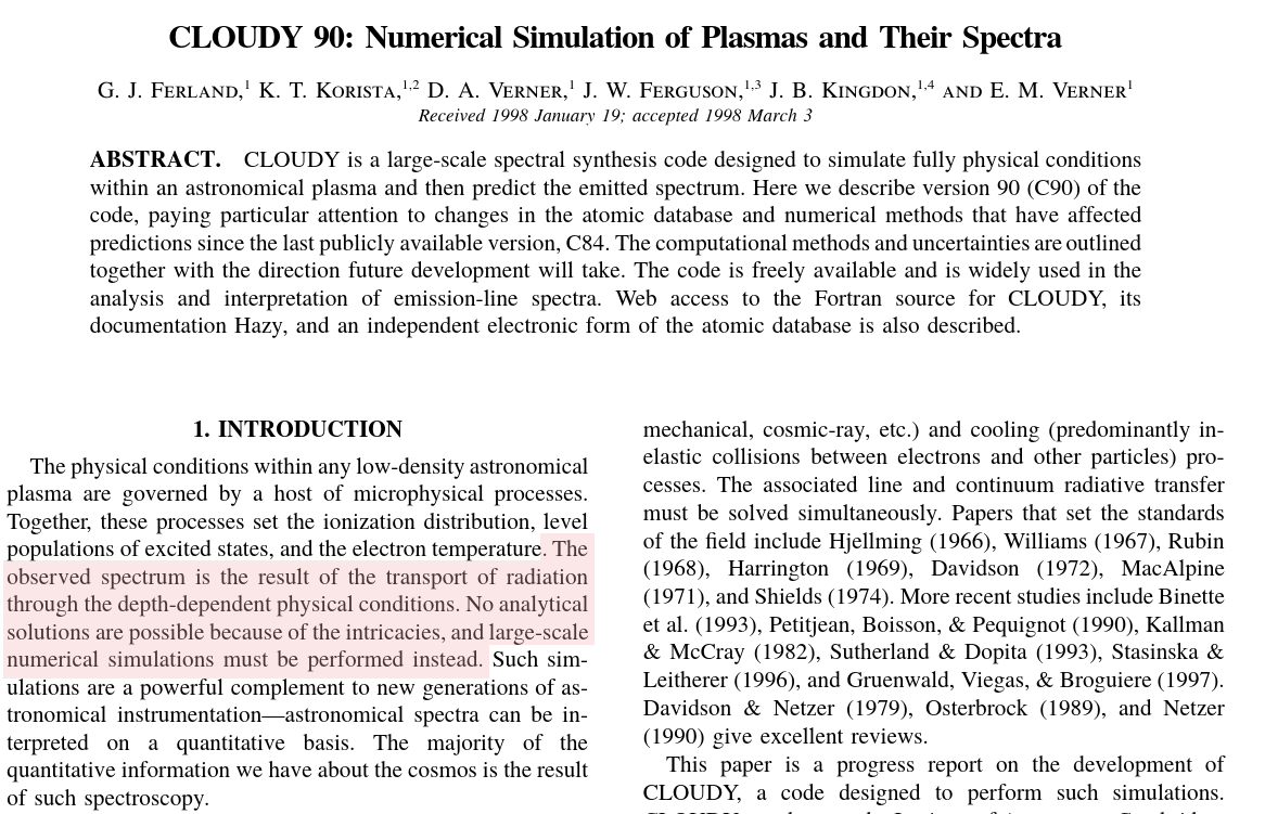
For more complicated situations, there is in general no simple analytic solution. Instead, one must use a computer to break space up into thin slices, apply the radiative transfer equation to each slice, and keep track of the resulting intensity. This becomes very complicated if the density, opacity, and source function change with position in the medium ... as, of course, they do in real stars. One can find a number of software packages designed to perform this task in the astronomical literature.
From the title page of
Fernald, G. J., et al., PASP 110, 761 (1998)
Look at a picture of the Sun carefully. Compare the appearance of the center of the solar disk to the edges.

Image of Sun thanks to
Big Bear Solar Observatory.
It looks brighter in the center, doesn't it? A color picture shows another difference:

Image copyright
Laurent Corp
The limbs of the Sun are not only dimmer than the center, they are redder, too. Why?
Part of the answer lies in the gradient of temperature within the solar photosphere. The deeper you go, the hotter it gets.
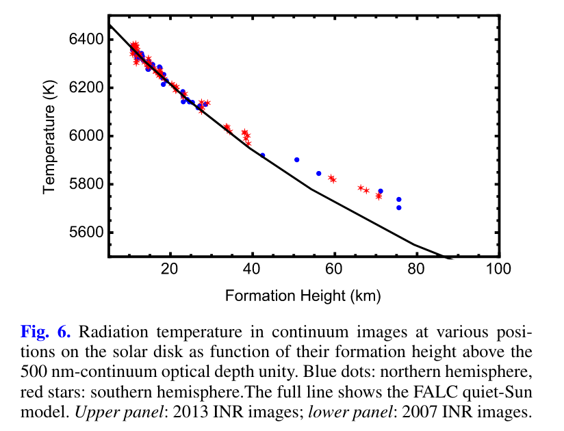
A portion of Figure 6 from
Faurobert, Balasubramanian, and Ricort, A&A 595, 71 (2016)
The other part of the answer involves optical depth. Light rays can escape from the Sun's photosphere when they are about 1 optical depth away from empty space. That means that we see photons which come from 1 optical depth "below the surface":
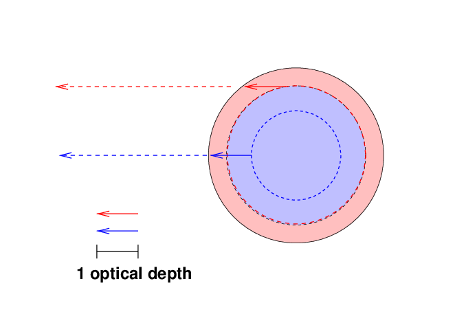
When we look at the center of the solar disk, we see light rays which are coming radially outwards. They originate relatively deep in the photosphere, where the temperature is relatively high; that means the source function S is (approximately) the blackbody function for a high temperature; say, T = 6100 K. When we look at the limbs, we see light rays which must skim through the photosphere at a shallow angle to reach the Earth. They originate in the upper reaches of the photosphere, where the temperature is somewhat lower; thus, the source function there might correspond to T = 5700 K.
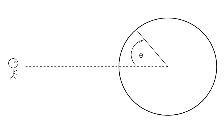
Since the source spectrum is (approximately) a blackbody in both instances, the radiation coming from the hot material near the center of the disk will be more intense (BRIGHTER) and have a shorter peak wavelength (BLUER). If we know exactly how temperature changes with radius, and how opacity and density change with radius, we can predict the change in surface brightness as a function of angular distance θ away from the center of the disk.
See the example in Section 9.3 of your textbook, which derives an expression of the form
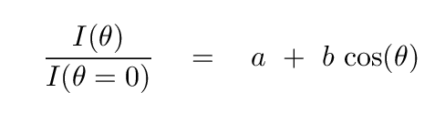
  Q:  If a star had NO limb darkening, but was the same brightness
           everywhere, what would be the value of the coefficient b?
The amount of limb darkening, represented in this simple formula as the coefficient b, must tell us something about the temperature structure of the star's outer atmosphere. If we could measure b for many different wavelengths, we might be able to figure out several properties of that atmosphere.
That's the theory -- what about real life? Well, we can MEASURE the brightness as a function of position very easily -- for the Sun:
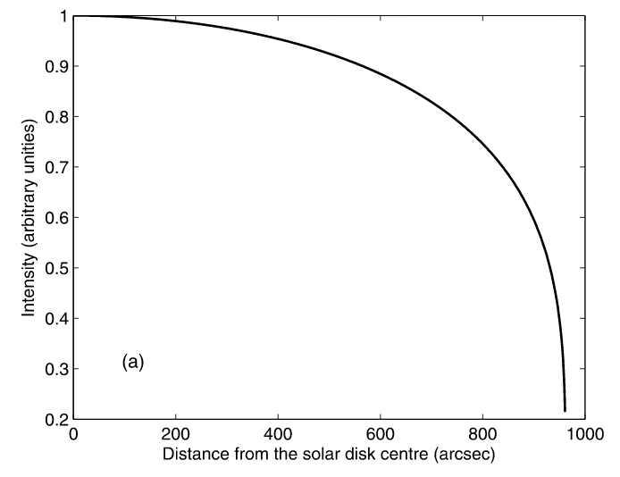
A portion of Figure 1 taken from
Thuillier et al., Solar Physics 268, 125 (2011)
Be careful when comparing limb darkening. Some studies, like the one above, use angular distance from the center of disk as the independent variable (on the horizontal axis); that's what one observes, after all. But in order to compare the results with theory, one must use the cosine of the angle as measured from the center of the Sun, as shown in the diagram below. Sometimes people call this quantity μ = cos(θ).
Now, apart from the Sun, there are very, very few stars which are big enough, and close enough, that astronomers can resolve their photospheres and measure their limb darkening. One of the very few which can be studied directly is the star Betelgeuse; but look at how few measurements we can make across its disk:
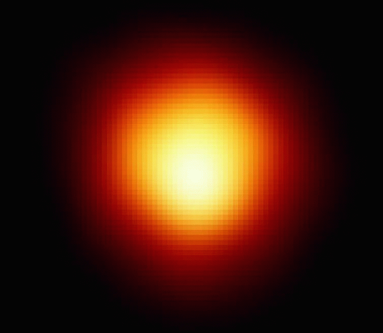
HST image of Betelgeuse courtesy of
A. Dupree (CfA), NASA, ESA
Apart from Betelgeuse and a few others, stars exhibit such small angular diameters that we have no way to resolve their disks, and so no way to measure their limb darkening. Rats! Limb darkening could tell us a lot about the properties of a stellar atmosphere. If only there was some clever way to see it ...
In the past 26 years, astronomers have spent a great deal of time, money, and effort measuring the tiny changes in a star's light caused by the transit of one of their planets crossing in front of its disk. If we could resolve the star and planet (we can't -- all we see is a single dot which changes in brightness), the event would look something like this.
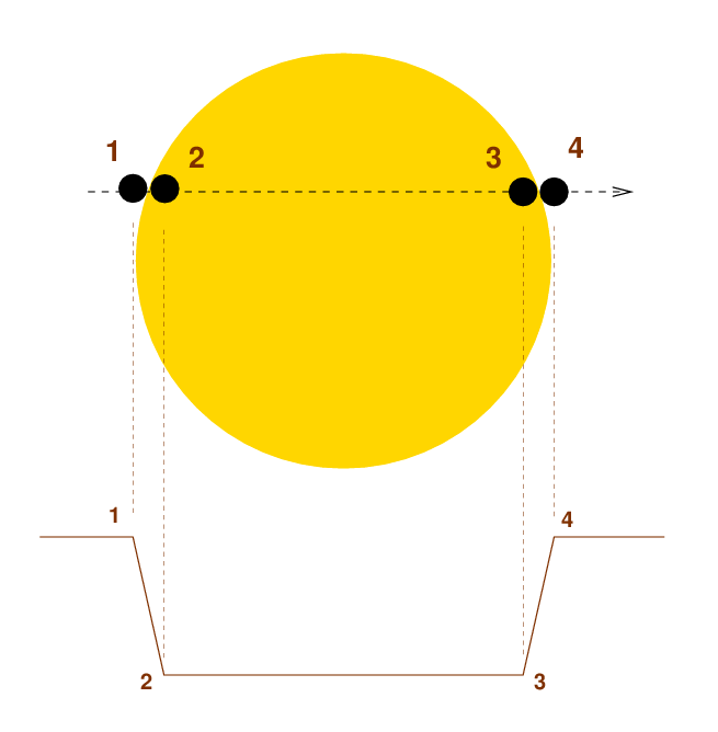
The light curve shown below the picture shows a graph of the star's brightness versus time. In the very simplified case of a star with constant brightness everywhere across its disk, the planet will block some constant amount of light once it fully enters and crosses the star. In this case, we'd expect the "bottom" section of a light curve to have a constant brightness -- the curve should be flat.
However, if you look at a REAL transit at different wavelengths, you'll see that its shape changes slightly. The figure below shows the transit of a planet around the star HD 209458 at wavelengths ranging from about 3000 Angstroms (purple, at bottom) to about 10000 Angstroms (red, at top).
![]()
Image taken from Figure 3 of
Knutson et al., ApJ 655, 564 (2007)
   Q:  What is the major difference between the shape
       of the curve at short vs. long wavelengths?
Yes, that's right: the transit light curve has a
It's the same star in each case -- so why the difference? Well, as discussed earlier, a real star like the Sun clearly does NOT show the same brightness across its entire face; instead, it's brighter near the center, and fades away toward the edges. Moreover, one important feature of this limb darkening is that it depends on the wavelength at which one observes: shorter wavelengths lead to stronger limb darkening.

The dip in light created by a transit shows us a sort of mirror image of the surface brightness of the star: the dip is deeper where the surface is brighter.
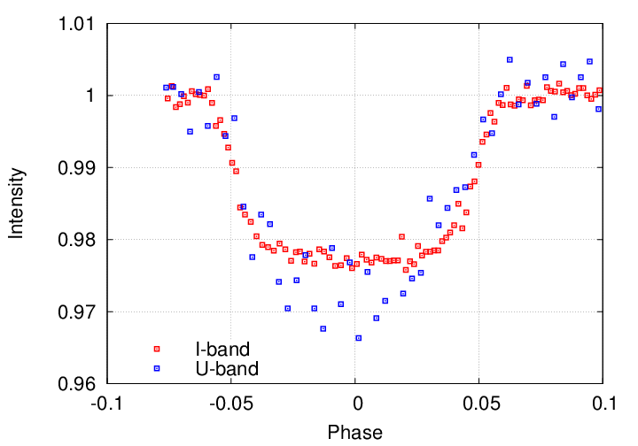
Transits of WASP 39 measured by
Ricci et al., PASP 127, 143 (2015)
Careful measurements of the transit at multiple wavelengths allow astronomers to determine the degree of limb darkening in a planet's host star; and that, in turn, can help them to pin down properties of the host star. Below are some examples of real transit light curves for a number of different stars, all observed with the Kepler satellite.

A portion of Figure B.2. from
Muller et al., A&A 560, 112 (2013)
Copyright © Michael Richmond.
This work is licensed under a Creative Commons License.