- parallax > 20 milliarcsec
- apparent g mag < 15
Because the Gaia archive site is misbehaving, I'll provide the datafiles that you haven't been able to extract. Each is in CSV format, parallax in column 10, phot_g_mean_mag in column 51, bp_rp in column 64.
- How many stars are in each dataset?
- Bob says "My subset has more stars than yours -- which proves that yellow stars must be more common in the Milky Way than red stars." Rey states that this might not be true, and suggests that they make a particular graph to find out. Make a graph showing the number of stars in shells of radius 1 pc, as a function of distance, in pc; make the horizontal axis limits from 0 to 15 pc. Plot both subsets on the graph, properly labelled.
- Based on this graph, who (if either) is correct?
- Now make a second graph, this time covering the range of distance from 0 to 50 pc. Can you explain the difference in the behavior of the yellow and red stars?
- In this second graph, what is happening to the red stars at a distance of about 25 pc?
- Based on all this information, was Bob's claim true or false? Explain your reasoning.
Based on values from Watson, W. D., ApJ 161, 139 (1970), let's assume that material in the solar core has
- opacity κ = 20 m2/kg
- density ρ = 2 x 10⁴ kg/m3
- What is the mean free path of a photon under these conditions?
- Assume that this mfp is constant throughout the Sun. How many steps will it take the photon to reach the surface of the Sun?
- How long will it take the photon to make this journey?
- How does this compare to the time it would take a photon to make the trip, if it were travelling through a vacuum?
Bonus! Are there any natural materials on the surface of the Earth with densities larger than that of the solar core?
Consider soot particles to be spheres of diameter d = 1 micron and density ρ = 100 kg/m3. We'll assume that light is absorbed if it touches one such sphere.
- What is the cross section area σ of a single soot particle?
- A fire emits soot particles into the air, causing an average of n = 1010 particles per cubic meter. What is the mean free path of photons through this soot-filled air?
- Suppose that there was no air or soot or any absorbing material, and light from the flashlight could travel freely to an observer's eyes. In that ideal case, how far away could Ruby detect Rick's messages?
- Once the air has filled with soot, what is the maximum distance at which a person could detect Rick's flashes of light?
Ranger Rick lives in a fire-control tower, elevated above the treetops. At night, he uses his trusty 10-watt flashlight to send messages in Morse code to his neighbor, Ranger Ruby. Assume that only 2 percent of the flashlight's power is emitted as photons of visible light (this is reasonable -- most turns into heat), and that the light is emitted isotropically (not so reasonable, but okay within an order of magnitude). Assume further that the human eye can detect a source of flux 109 photons per second per square meter (this is roughly correct).
Use the image sun_big_bear.fits as our starting point. It is an image of the Sun in broadband optical light, taken by astronomers at the Big Bear Solar Observatory. The image is in FITS format, which can analyzed with many different astronomical image processing packages; among them is a package called ds9.
- Download the image to your own computer. Display it, using ds9 or any other program of your choice. Verify that it looks like the Sun, and that it is brighter at the center than the edges.
- Measure data along a horizontal slice through the middle
of the Sun, yielding a set of about 830 or so
pairs of values: (pixel x coord, intensity).
You may use any software you wish to do this;
instructions for using ds9 follow.
- run ds9
- display the image using File -> Open -> sun_big_bear.fits
- prepare to measure, by choosing Edit -> Region
- in order to make a slice through the image, choose Region -> Shape -> Projection
- left-click and drag a line horizontally across the equator of the solar image. A new window with a graph showing intensity as a function of position should pop up.
- In this new window, save the data via File -> Save Data -> (type a name here) . This should create a text file with two columns, pixel value and intensity.
- Make a plot showing intensity as a function of pixel position. Be sure to put proper labels on the axes
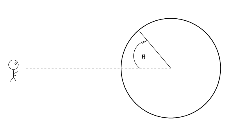
- Now, compute the angle θ away from the center of the disk for each measured point. As shown in the figure above, this angle should be 0 at the center of the disk, and 90 degrees (or π/2 radians) at the edge of the disk. Make a second plot, this one showing intensity as a function of cos(θ). The x-axis should run from 0 to 1.
- On this graph, you should see a nearly straight line running down and to the left, and then perhaps dropping more rapidly toward zero. Fit a line to the linear portion of the graph, and measure the slope.
- As discussed in class and in section 9.3 of your text,
theory states that under certain assumptions,
the measured intensity should vary in a simple
manner:
I(θ) = (2/5) I0 + (3/5) I0 cos(θ)
Does your data follow this simple equation? Discuss.