Working with Matrices

This section introduces you to other ways of creating matrices. The SCILAB is most powerful while handling matrices it allows you to manipulate the matrix as a whole.

Generating Matrices

SCILAB provides three functions that generate basic matrices:

	zeros All zeros
	ones All ones
	rand Random elements (either normal or uniform)

Some examples

zeros(3,3)

        ans =

        ! 0. 0. 0. !
        ! 0. 0. 0. !
        ! 0. 0. 0. !

4*ones(3,3)

        ans =

        ! 4. 4. 4. !
        ! 4. 4. 4. !
        ! 4. 4. 4. !

rand(4,4,'normal')

        ans =

        ! 1.4739763 .2546697 - 1.0327357 .0698768   !
        ! .8529775 - .6834217 - .9239258 - 1.3772844 !
        ! .7223316 .8145126 2.7266682 - .1728369     !
        ! .6380837 - .1884803 - 1.7086773 - .6019869 !

Load

The load command reads binary files containing matrices generated by earlier SCILAB sessions, or reads text files containing numeric data. The text file should be organized as a rectangular table of numbers, separated by blanks, with one row per line, and an equal number of elements in each row. For example, outside of SCILAB, create a text file containing these four lines:

magic =

  ! 16.0     3.0     2.0    13.0 !
  ! 5.0    10.0    11.0     8.0  !
  ! 9.0     6.0     7.0     12.0 !
  ! 4.0    15.0    14.0     1.0  !

Store the file under the name magic_square.dat.

save magic_square

Then the command

	load magic_square.dat

Reads the file and creates a variable, magic, containing our example matrix.

SCI-Files

You can create your own matrices using sci-files, which are text files containing SCILAB code. Just create a file containing the same statements you would type at the LAB command line. Save the file under a name that ends in .sci.

Note: To write a sci-file open a textpad or notepad and write the code in the text file. Then save the file with the extension <filename.sci>. On the command window go the file control button and click the exec option and choose the file you want to execute.

For example,

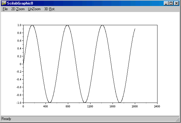
A sci-file which will plot a sine wave, (use notepad to write the code)

// this is comment line

// sci-file to plot sine wave

time = 0:.01:20;

plot(sin(time));

save this file as My_prog.sci and run the program as mentioned above. You can also run the program in command window by typing,

exec('Pathname')

i.e.,

exec('E:\Scilab-2.6\work\My_prog.sci')

On executing the program you will see the Sine wave in the figure window as show below.

Concatenation

Concatenation is the process of joining small matrices to make bigger ones. In fact, you made your first matrix by concatenating its individual elements. The pair of square brackets, [], is the concatenation operator.

For example,

a = [ 1 2 3 ]; b= [ 4 5 6]; c = [ 7 8 9];

d= [ a b c]

d =

! 1. 2. 3. 4. 5. 6. 7. 8. 9. !

Deleting Rows and Columns

You can delete rows or columns from a matrix by using just a pair of square brackets.

For example,

s = [ 1 2 3 4; 5 6 7 8; 9 10 11 12 ]

        s =

        ! 1. 2. 3. 4.       !
        ! 5. 6. 7. 8.       !
        ! 9. 10. 11. 12. !

s(:,2) =[]

produces

        s =

        ! 1.   3.   4. !
        ! 5.   7.   8. !
        ! 9. 11. 12. !

If you delete a single element from a matrix, the result isn't a matrix anymore.

So if you type expressions like ,

s(1,3) =[]

!--error 15
submatrix incorrectly defined

will result in error.

However, using a single subscript deletes a single element, or sequence of elements, and reshapes the remaining elements into a column vector. So,

   s(2:2:9) = [ ]


results in

s  =

!   1.  !
!   9.  !
!   6.  !
!   3.  !
!   11. !
!   4.  !
!   8.  !
!   12. !