Graphics

SCILAB has extensive facilities for displaying vectors and matrices as graphs, as well as annotating and printing these graphs. This section describes a few of the most important graphics functions and provides examples of some typical applications.

It is possible to use several graphics windows ScilabGraphicx x being the number used for the management of the windows, but at any time only one window is active. On the main SCILAB window the button Graphic Window x is used to manage the windows : x denotes the number of the active window, and we can set (create), raise or delete the window numbered x : in particular we can directly create the graphics window numbered 10. The execution of a plotting command automatically creates a window if necessary.

There are 4 buttons on the graphics window:

	`3D Rot.`: for applying a rotation with the mouse to a 3D plot. This button is inhibited for a 2D plot. For the help of manipulations (rotation with specific angles ...) the rotation angles are given at the top of the window.
	`2D Zoom`: zooming on a 2D plot. This command can be recursively invoked. For a 3D plot this button is not inhibited but it has no effect.
	`UnZoom`: return to the initial plot (not to the plot corresponding to the previous zoom in case of multiple zooms). These 3 buttons affecting the plot in the window are not always in use; we will see later that there are different choices for the underlying device and zoom and rotation need the record of the plotting commands which is one of the possible choices (this is the default).
	`File`: this button opens different commands and menus. The first one is simple : `Clear` simply rubs out the window (without affecting the graphics context of the window). The command `Print...` opens a selection panel for printing. Under Unix, the printers are defined in the main scilab script `SCIDIR/bin/scilab` (obtained by ``make all'' from the origin file `SCIDIR/bin/scilab.g`). The `Export` command opens a panel selection for getting a copy of the plot on a file with a specified format (Postscript, Postscript-Latex, Xfig). The `save` command directly saves the plot on a file with a specified name. This file can be loaded later in Scilab for replotting. The `Close` is the same command than the previous `Delete Graphic Window` of the menu of the main window, but simply applied to its window (the graphic context is, of course deleted).

Creating a Plot

The plot function has different forms, depending on the input arguments. If y is a vector, plot(y) produces a piecewise linear graph of the elements of y versus the index of the elements of y. If you specify two vectors as arguments, plot(x,y) produces a graph of y versus x.

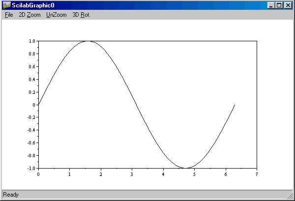
For example, to plot the value of the sine function from zero to 2, use

t = 0:%pi/100:2*%pi;

y = sin(t);

plot(t,y);

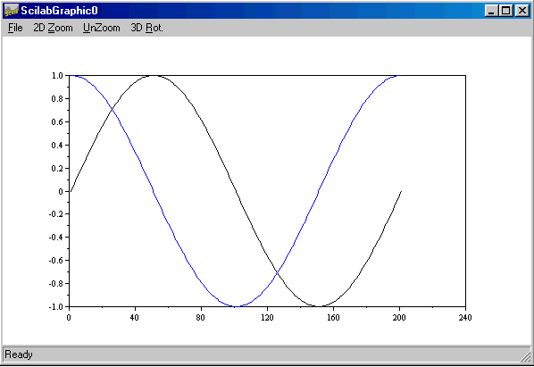
Multiple x-y pairs create multiple graphs with a single call to plot. SCILAB automatically cycles through a predefined (but user settable) list of colors to allow discrimination between each set of data. For example, these statements plot two related functions of t, each curve in a separate distinguishing color:

For example,

plot([sin(t);cos(t)]);

produces,

Subplots

The subplot function allows you to display multiple plots in the same window or print them on the same piece of paper.

Typing,

subplot(m,n,p)
subplot(mnp)

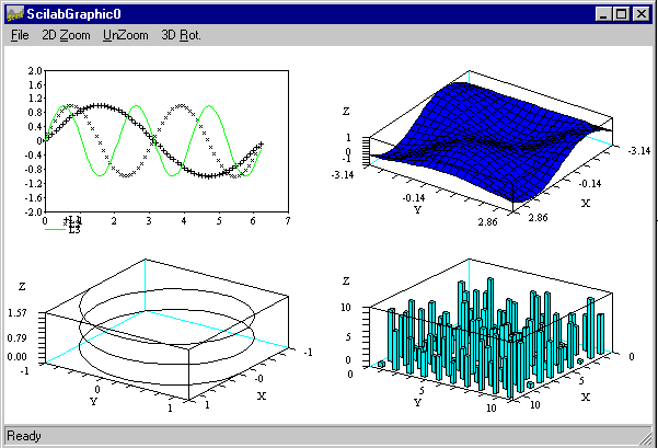
breaks the figure window into an m-by-n matrix of small subplots and selects the pth subplot for the current plot. The plots are numbered along first the top row of the figure window, then the second row, and so on. For example, to plot data in four different subregions of the figure window,

        subplot(221)
        plot2d()
        subplot(222)
        plot3d()
        subplot(2,2,3)
        param3d()
        subplot(2,2,4)
        hist3d()

produces,

Controlling Axes

Ordinarily, SCILAB finds the maxima and minima of the data and chooses an appropriate plot box and axes labeling. The axis function overrides the default by setting custom axis limits,

square(xmin xmax ymin ymax)

The requested values xmin, xmax, ymin, ymax are the boundaries of the graphics frame and square changes the graphics window dimensions in order to have an isometric plot.

By typing,

xset("default")

The original default size will be used for the graphic windows.

Axes Labels and Titles

The x-axis and y-axis labels and caption (Title) of the plot can be given in the plot function itself. typing

plot(x,y,[xcap,ycap,caption])

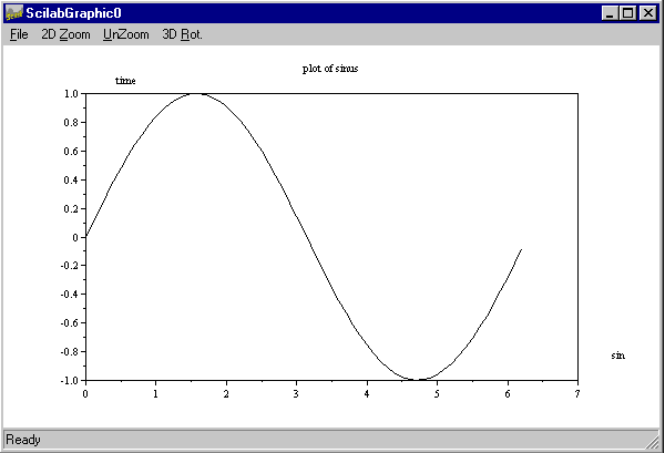
For example,

        x=0:0.1:2*%pi;
        // simple plot
        plot(sin(x))
        // using captions
        xbasc()
        plot(x,sin(x),"sin","time","plot of sinus")

This produces,

Printing Graphics

The Print option on the File menu and the print command both print MATLAB figures. The Print menu brings up a dialog box that lets you to print the figure.

Window to Paper

The simplest command to get a paper copy of a plot is to click on the print button of the SCILAB graphic window.

Creating a Postscript File

The simplest way to get a Postscript file containing SCILAB plot is :

driver('Pos') // selects a graphics driver

xinit('foo.ps') // initialization of a graphics driver

plot3d1(); // demo of plot3d1

xend() // closes graphics session

driver('Rec')

plot3d1()

xbasimp(0,’foo1.ps’) //send graphics to a Postscript printer or in a file

The Postscript files (foo.ps or foo1.ps ) generated by SCILAB cannot be directly sent to a Postscript printer, they need a preamble. Therefore, printing is done through the use of Unix scripts or programs which are provided with SCILAB. The program Blpr is used to print a set of SCILAB

Graphics on a single sheet of paper and is used as follows :

Blpr string-title file1.ps file2.ps > result

You can then print the file result with the classical Unix command :

lpr -Pprinter-name result

or use the ghostview Postscript interpreter on your Unix workstation to see the result.