Example: the Temperature Profile of the Earth's Atmosphere

When it makes sense to leave a program in one piece ...

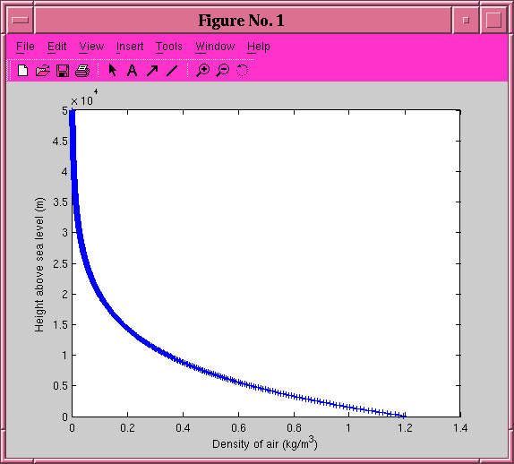
Let's consider the atmosphere of the Earth; you're using it in your simulation of the cannonball this week. Now, the density of the atmosphere is a pretty simple function of altitude:

      rho(height)  =   (1.21 kg/m^3) * exp(-height/8000 m)

So one can write a simple routine to plot the density as a function of height from, say, sea level to an altitude of 100 km. It might look like this:

plot_air_density.sci

The central loop in this program is short and sweet, easy to understand at a glance:


  for  i = 1 : num_pieces 
    altitude = start_altitude + i*delta_altitude;
    density = rho_nought * exp(-altitude/scale_height);

    y(i) = altitude;
    x(i) = density;
  end

In this case, the calculation of air density is so simple that it may not make sense to move it to a function of its own; leaving it in the main loop is fine. But what if the physical quantity behaves in a more complicated manner?

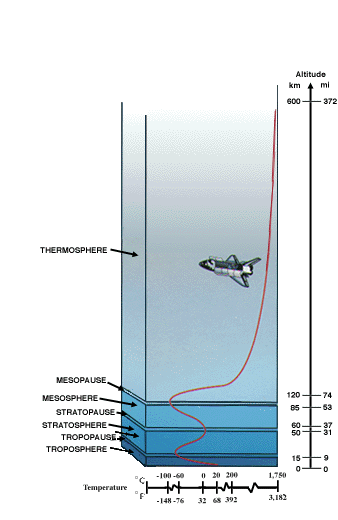
When it makes sense to break a program into functions ....

The temperature of the Earth's atmosphere, for example, is NOT a simple function of altitude:

We can approximate this complicated behavior by breaking the atmosphere into a set of layers, and using a simple function within each layer. But that makes the main loop of a program a lot less easy to grasp at a glance:


  for  i = 1 : num_pieces 
    altitude = start_altitude + i*delta_altitude;

    // for the troposphere ...
    if (altitude < troposphere_boundary)
      xx = altitude - 0;
      temperature = a1 + b1*xx;

    // for the lower stratosphere
    elseif (altitude < lower_strat_boundary)
      xx = altitude - lower_strat_boundary;
      temperature = a2 + b2*xx;
  
    // for the upper stratosphere
    else 
      xx = altitude - upper_strat_boundary;
      temperature = a3 + b3*xx + c3*(xx*xx);
    end

    y(i) = altitude;
    x(i) = temperature;
  end

In this case, we can make the main loop much shorter and easier to understand by creating a function to do all the dirty work. The main loop then might look like so:


  for  i = 1 : num_pieces 
    altitude = start_altitude + i*delta_altitude;
    temperature = air_temperature(altitude);

    y(i) = altitude;
    x(i) = temperature;
  end

And, after the end of the main program, the source code might contain a function which starts something like this:

//////////////////////////////////////////////////////////////////////////
//
function temp = air_temperature(altitude)
//
// Calculate the temperature of the Earth's atmosphere (in degrees F)
//   as a function of height (in meters).  
//
// Arguments:      altitude    (input)     height above sea level (meters)
//
//                 temp        (output)    temperature of air (degrees F)
//

   ....

In-class exercise

Go to this NASA site to find a simple approximation to the temperature of air in the lower layers of the atmosphere.

http://www.grc.nasa.gov/WWW/K-12/airplane/atmos.html

Write a Scilab program in a source code file called plot_air_temperature.sci. Your program should have two functions:

a main function called plot_air_temperature
a secondary function called air_temperature, which takes altitude (in meters) as input and returns air temperature (in degrees F) as output

The program should calculate temperature at altitudes from sea level to 50,000 meters, in steps of 100 m. It should generate a graph like the one for density above, showing altitude (in meters) on the x-ais and temperature (in degrees F) on the y-axis. You can check your graph against the picture of temperature versus altitude in the NASA graphic above.

When you think it works, call me over to check it. If I approve, print onto paper

a copy of your program
a copy of your graph of altitude versus temperature

and hand them to me.

For more information

A model of the Earth's atmosphere from NASA's Glenn Research Center.