Finding Roots by "Closed" Methods

One general approach to finding roots is via so-called "closed" methods.

What is a "closed" method?
The Bisection Technique
Example of the Bisection Technique
Termination Conditions
The False Position Technique

See Chapter 5 of your textbook for more information on these methods.

Closed methods

A closed method is one which starts with an interval, inside of which you know there must be a root. At each step, the method continues to produce intervals which must contain the root, and those intervals steadily (if slowly) shrink. These methods are guaranteed to find a root within the interval, as long as the function is well-behaved.

Open methods can be much faster, but they give up this certainty.

The two closed methods discussed here also require only that you be able to evaluate the function at some point; they do not require that you also be able to evaluate the function's derivative.

The Bisection Technique

Given some function f(x) which is real and continuous, and given some interval [x1, x2] inside of which you want to check for a root, do the following:

Calculate f(x1)
Calculate f(x2)
Check to see if they have the same sign. If so, there may be no root between them. Quit
If they have opposite signs, then
1. Pick a point, x_new, halfway in between the two ends
2. Look at the sign of f(x_new)
  1. If it's the same as f(x1), the root lies between x_new and x2; so set x1 = x_new
  2. If it's the same as f(x2), the root lies between x1 and x_new; so set x2 = x_new
  3. If f(x_new) = 0, then you're done
3. Go to step "a"

Good things about the bisection method:

it's certain: the root MUST be inside the range
it ALWAYS converges
each iteration improves the estimate by a known about (how much?)
only requires evaluation of function, not derivative

Bad things about the bisection method:

may converge more slowly than some other methods

Example of Bisection method

Let's look at a specific example of the bisection technique:

     find a root of the equation   y = x^2 - 4    on interval [0, 5]
 
             stop when relative fractional change is 1e-5

The exact root is 2, of course. How quickly can we find it, to within the given termination criterion?

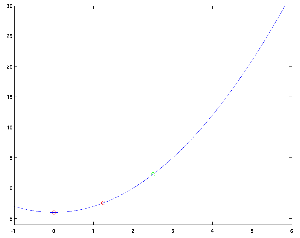
Let's watch the method in action, one step at a time. First, we need to calculate the value of the function at the bottom of the interval (x1 = 0), and the top of the interval (x2 = 5). We also make our first guess: the midpoint of the interval, x_new = 2.5, and evaluate the function there, too.

Now, looking at the sign of the function at each of these points, we see that

the sign is negative at x1
the sign is positive at x_new
the sign is positive at x2

The root must lie somewhere between x1 and x_new, because the function MUST change sign at a root. So, we leave x1 = 0, but move x2 to the current midpoint. Our interval is now [0, 2.5].

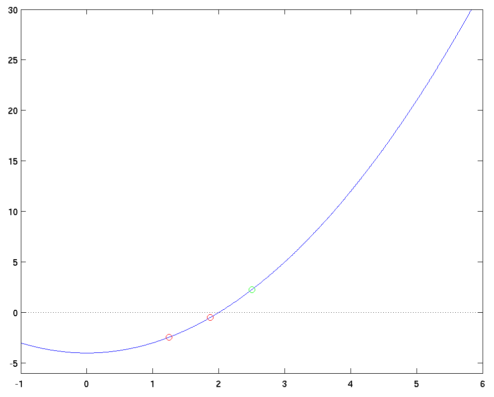
We now repeat the bisection's basic step: find the midpoint of the current interval (x_new = 1.25), and look at the sign of the function at the endpoints and the midpoint.

This time, the function changes value between the midpoint x_new = 1.25 and the upper bound x2 = 2.5. That means that we'll discard the old lower bound, and re-set it so that x1 = 1.25 for the next step. Our interval is now [1.25, 2.5].

Going back to the top of the loop, we find the midpoint x_new = 1.875, and evaluate the function here and at the endpoints.

It looks like we'll have to move the lower bound again in the next step ...

You can watch the progress of the bisection method in these movies:

Movie with fixed limits (slow version)
Movie with fixed limits (fast version)
Movie which zooms in after each step (it only shows the first 4 iterations, but you'll get the idea)

Here's a table showing the method in action:

                 lower      value at       upper       value at      fractional
 iter            bound     lower bound     bound      upper bound      change
------------------------------------------------------------------------------
iter     0   0.0000000e+00 -4.0000e+00   5.0000000e+00 2.1000e+01   1.0000e+00 
iter     1   0.0000000e+00 -4.0000e+00   2.5000000e+00 2.2500e+00   1.0000e+00 
iter     2   1.2500000e+00 -2.4375e+00   2.5000000e+00 2.2500e+00   3.3333e-01 
iter     3   1.8750000e+00 -4.8438e-01   2.5000000e+00 2.2500e+00   1.4286e-01 
iter     4   1.8750000e+00 -4.8438e-01   2.1875000e+00 7.8516e-01   7.6923e-02 
iter     5   1.8750000e+00 -4.8438e-01   2.0312500e+00 1.2598e-01   4.0000e-02 
iter     6   1.9531250e+00 -1.8530e-01   2.0312500e+00 1.2598e-01   1.9608e-02 
iter     7   1.9921875e+00 -3.1189e-02   2.0312500e+00 1.2598e-01   9.7087e-03 
iter     8   1.9921875e+00 -3.1189e-02   2.0117188e+00 4.7012e-02   4.8780e-03 
iter     9   1.9921875e+00 -3.1189e-02   2.0019531e+00 7.8163e-03   2.4450e-03 
iter    10   1.9970703e+00 -1.1710e-02   2.0019531e+00 7.8163e-03   1.2210e-03 
iter    11   1.9995117e+00 -1.9529e-03   2.0019531e+00 7.8163e-03   6.1013e-04 
iter    12   1.9995117e+00 -1.9529e-03   2.0007324e+00 2.9302e-03   3.0516e-04 
iter    13   1.9995117e+00 -1.9529e-03   2.0001221e+00 4.8830e-04   1.5260e-04 
iter    14   1.9998169e+00 -7.3239e-04   2.0001221e+00 4.8830e-04   7.6295e-05 
iter    15   1.9999695e+00 -1.2207e-04   2.0001221e+00 4.8830e-04   3.8146e-05 
iter    16   1.9999695e+00 -1.2207e-04   2.0000458e+00 1.8311e-04   1.9073e-05 
iter    17   1.9999695e+00 -1.2207e-04   2.0000076e+00 3.0518e-05   9.5368e-06

The result is 1.99998855590820, which is indeed close to 2.0.

Termination conditions

Now, if you try to implement the method shown above, you may discover that your program never stops running -- or runs for a long, long time. Ooops. The algorithm has only one termination condition: if you find the EXACT root, then quit; otherwise, keep going. In most cases, the computer can't represent the EXACT root, and so you may never find it.

You should always include a termination condition in a root-finding function ... and you should always think about termination conditions in any iterative method. There are a number of possibilities, but all of them require that you pick some small value epsilon.

if the absolute value of the function falls below epsilon, quit. We're looking for a root, a place where f(x) equals zero, so
```
         | f(x) |  <  epsilon
```
might make sense; we're probably close ...
if the latest value of x is within epsilon of the true root value, then quit:
```
         | x_new - x_true | < epsilon
```
Unfortunately, we don't know the true root x_true. Oops.
if the latest value of x is only a teensy bit different from the previous value, then quit:
```
         | x_new - x_prev | < epsilon
```
This is reasonable ...
if the fractional change in x is very small, then quit:
```
         | x_new - x_prev |
         | -------------- |   <  epsilon
         |     x_new      |
```
This is one of the most commonly used criteria. Note that bad things can happen if the root is near zero, because we will then be dividing by a very small number.

False Position Technique

The basic idea here is to use an estimate for the new value of the root which is better than the midpoint of the range. As before, it starts with a boundary for which the function is positive at one end and negative at the other. The method assumes that the function changes linearly from one end to the other, and calculates the value of x_new at which that linear approximation crosses zero.

An algorithm for this method looks almost identical to the one above for the Bisection method, but in Step 4a, instead of

If they have opposite signs, then
1. Pick a point, x_new, halfway in between the two ends

you make a linear fit to the function between the two ends, and find the spot where that fit crosses zero:

If they have opposite signs, then
1. Pick a point, x_new, at which a linear fit between f(x1) and f(x2) equals zero

You can interpolate from either end; the textbook works out the calculation of x_new working backwards from the upper end x2.

Good things about the false position method

it ALWAYS converges
it usually converges more quickly than the Bisection method
only requires evaluation of function, not derivative

Bad things about the bisection method:

each iteration improves the estimate by an unknown amount
may converge very slowly for some functions

Last modified 3/26/2002 by MWR.