 Copyright © Michael Richmond.
This work is licensed under a Creative Commons License.
Copyright © Michael Richmond.
This work is licensed under a Creative Commons License.
Today, we're going to investigate the properties of a very particular combination of vibrations with slightly different frequencies.
But to start, let's look at a vibration with a single, pure frequency. How about ω1 = 1 rad/s? That's simple enough. Over 20 seconds, this vibration completes several cycles.
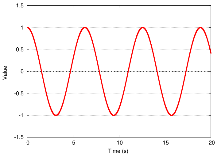
Q: What is the period of this oscillation?
As you will see soon, combining vibrations with slightly different frequencies will cause interesting effects. In order to produce some of these effects on relatively short timescales -- so that we don't have to plot hours and hours of measurements to see the effects -- it will help to combine very high frequencies.
So, let's set our new baseline to ωh = 1000 times ω1 = 1000 rad/s. In the graph below, the original frequency is show in red, and the new, high frequency is shown in green.

Q: Can you see the variations in the high-frequency vibration?
No? Well, let's zoom in to a smaller timescale.

Okay, now you can see the variations in the high frequency vibration.
Now, if you look at a graph of a single frequency, you will see periodic variations in value (look at the red line in the diagram below), but over longer stretches of time, the value remains exactly the same (look at the green line in the diagram below). In other words, we can't really identify any special time associated with a single frequency.
However, if we add together several frequencies, then the situation changes. If the frequencies are relatively similar, then the combination will yield obvious variations in the size of the "envelope" of the sum.
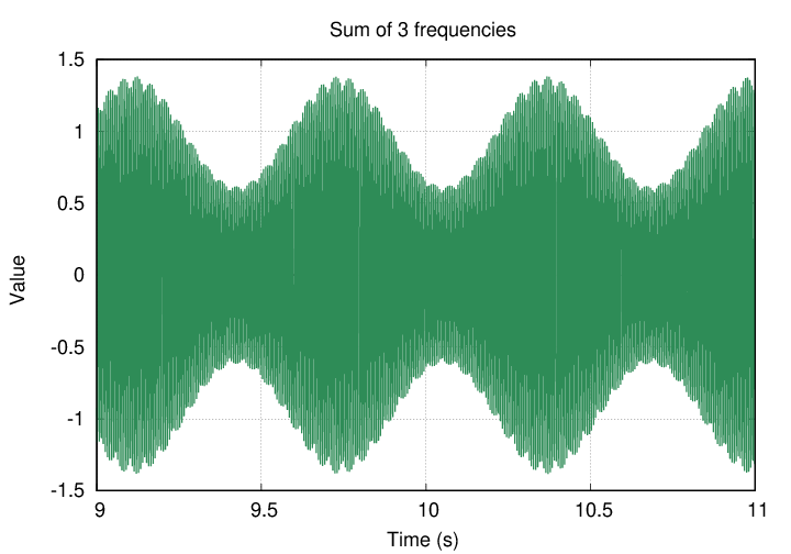
For example, if I add together three high-frequency vibrations which are centered on ωh,
then the sum will still oscillate at roughly ωh, but the overall size of the result will change over a number of cycles. In a zoomed-in view, the sum looks like this:

Zooming out a bit, one can see the periodic fluctuations in the "envelope" of the sum.
  Q:  What is the name given to this slow variation in the
            sum of several high frequencies?
Right. We call these slow variations "beats", and musicians who play together must tune their instruments together to avoid them.
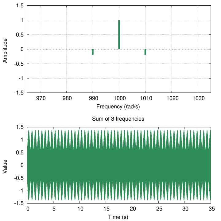
Let's create a standard graph to illustrate the addition of several frequencies centered on ωh. In the upper panel will be a frequency spectrum, showing the number of frequencies being combined, and their relative amplitudes; in the lower panel will be picture of the resulting vibration over 35 seconds of time. For our example of vibrations with 990, 1000, 1010 rad/s, the graph looks like this.
But suppose that I divide that same range of frequencies, 990 to 1010, into 9 components, rather than 3.
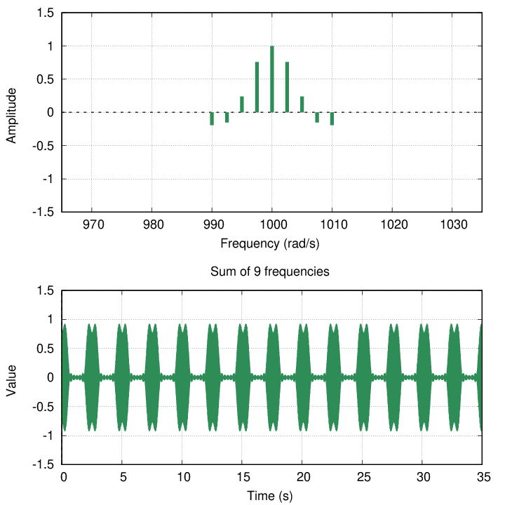
Hmmm. The sum is starting to break up into sections of time when the result has a large amplitude, and stretches of time when the result is nearly zero. Let's call the short bursts of high amplitude pulses.
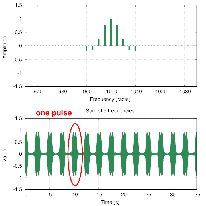
Q: How far apart in time are these pulses?
Each pulse is about 2.5 seconds away from its neighbors.
If we look at one pulse in detail, we see that it has some particular width in time. In this case, it appears to be roughly one second long.

         width of freq       number of freq     time between pulses
    ------------------------------------------------------------------
         +/-   10  rad/s          9                   2.5  s
If we divide the range of 990 to 1010 -- which we might refer to as 1000 +/- 10 rad/s -- into more frequencies, and add them together, then the result changes.

Fill in the table below.
         width of freq       number of freq     time between pulses
    ------------------------------------------------------------------
         +/-   10  rad/s          9                   2.5  s

         +/-   10  rad/s         39
And if we add even more components within this fixed range, 1000 +/- 10 rad/s, then the pulses become spaced even farther apart in time.

Fill in the table below.
         width of freq       number of freq     time between pulses
    ------------------------------------------------------------------
         +/-   10  rad/s          9                   2.5  s

         +/-   10  rad/s         39

         +/-   10  rad/s         99
In theory, if we could add together a very large number of very-closely-spaced frequencies, we could create a series of pulses which were spaced very widely.
Or, if we push things to the limit, if we could add together an INFINITE number of closely-spaced-frequencies, we might be able to create a single pulse which didn't repeat for an INFINITE length of time. In other words, we could combine a bunch of periodic functions to create a NON-PERIODIC result.

Image of Jackie Chan courtesy of
knowyourmeme.com
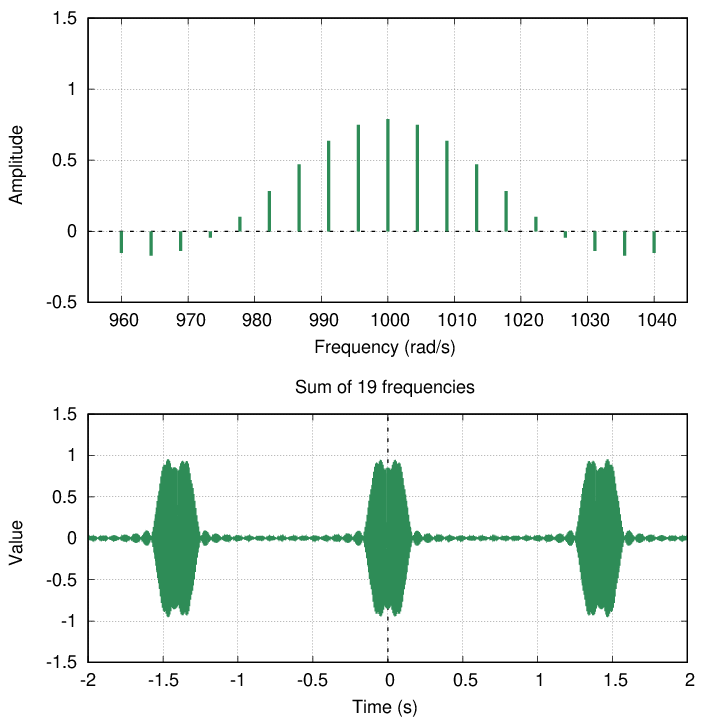
But let's look at a different property of these "pulses:" the duration of each one. In other words, the length of time that each pulse lasts. In all the examples below, I'll combine 19 frequencies centered on ωh = 1000 rad/s. Let's measure the width of frequencies used to create the pulse, and the duration = width in time of the resulting pulse.
I'll do the first example.
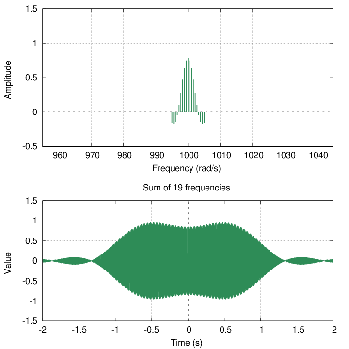
               width of frequency        width of pulse
           --------------------------------------------------
                  +/-   5   rad/s          +/-   1.3  s

           --------------------------------------------------
Okay, your turn. Let's make the range of frequencies broader.
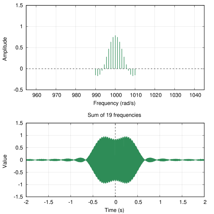
               width of frequency        width of pulse
           --------------------------------------------------
                  +/-   5   rad/s          +/-   1.3  s

                  +/-                      +/-

           --------------------------------------------------
               width of frequency        width of pulse
           --------------------------------------------------
                  +/-   5   rad/s          +/-   1.3  s

                  +/-                      +/-

                  +/-                      +/-

           --------------------------------------------------
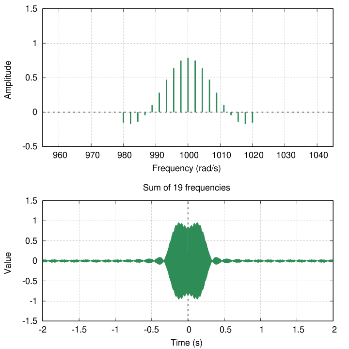
Are you sensing a pattern?
Let's do one more example.
               width of frequency        width of pulse
           --------------------------------------------------
                  +/-   5   rad/s          +/-   1.3  s

                  +/-                      +/-

                  +/-                      +/-

                  +/-                      +/-

           --------------------------------------------------
  Q:  Write a mathematical relationship which connects the
             width of frequencies added together to the width of
             the resulting pulse.
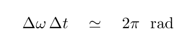
The basic idea is that as the range of frequencies increases, the duration in time decreases proportionally. There are several ways to write this in an equation, but one is

In this particular instance, the constant is a familiar value:
Now, does this sort of relationship look familiar to you? Have you seen anything similar in your physics classes so far?
It should. Back in the early twentieth century, physicists studying atoms and sub-atomic particles found that there was a fundamental limitation to their ability to measure the properties of any one particular particle. It required a very long time to measure the energy of a particle precisely; conversely, if a particle decayed after a short lifetime, its energy could not be measured accurately.
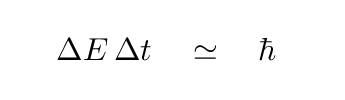
And, gosh, the energy of a photon is related to its frequency, isn't it?
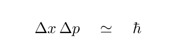
You may be more familiar with another uncertainty relationship, which connects the uncertainty in the position of a particle to the uncertainty in its momentum.
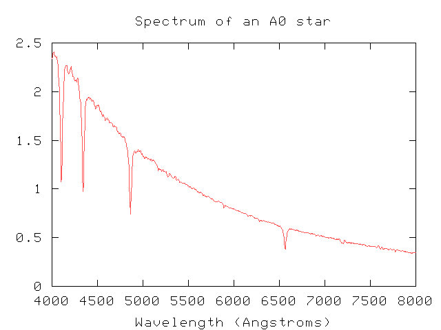
Astronomers have been breaking the light from stars into spectra for about 170 years now. In the optical part of the spectrum, a typical star's light shows a blackbody curve, with absorption lines superimposed on the continuum.
In 2016, a paper appeared which claimed that a small fraction of stars in a very large survey showed peculiar features: periodic variations in intensity as a function of wavelength, which corresponded to periodic variations in intensity as a function of time.
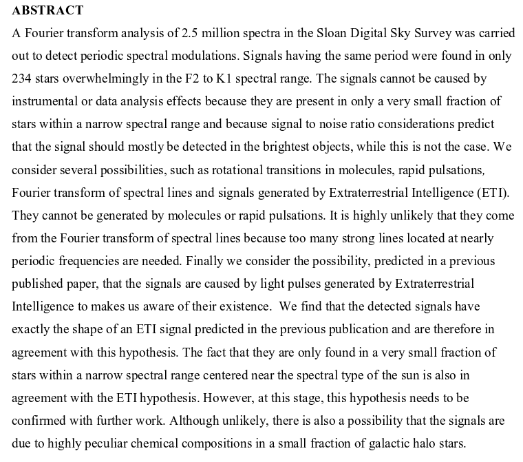
Abstract of
Borra and Trottier, PASP 128, 11401 (2016)
The basic idea was that if one performed a specific type of Fourier analysis of the starlight -- similar to computing the coefficient of the Fourier series for each particular wavelength -- then it revealed a peculiar feature in a tiny fraction of all stars. The power spectrum of a typical star looked like this: note the long stretch of data in the middle of the graph, where all the values are low.

Figure 6 taken from
Borra and Trottier, PASP 128, 11401 (2016)
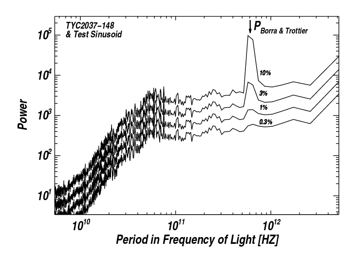
but that of some stars -- often those similar to the Sun -- showed a feature corresponding to a certain frequency. In the graph below, this feature is the narrow line extended upward near bin N=770.
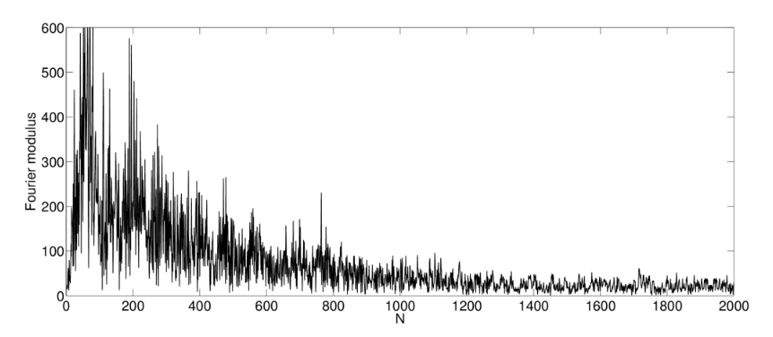
Figure 8 taken from
Borra and Trottier, PASP 128, 11401 (2016)
This feature, according to the authors, meant that the spectra of some stars showed significant wiggles over scales in wavelength of 5 to 6 nm.
In other words, periodic variations in the intensity of starlight in a spectrum. Shown below is one small stretch of the spectrum of a star between 461 and 428 nm, with a sine curve of the postulated period drawn for comparison.
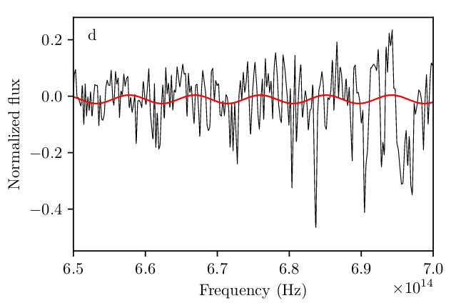
Figure 1d taken from
Hippke, arXiv 1901.00523 (2019)
Borra and Trottier considered several physical sources for this sort of spectral feature, but discarded each one as improbable. They suggested that one explanation might be
Finally, we considered the possibility that the signals are caused by intensity pulses generated by Extraterrestrial Intelligence (ETI), as suggested by Borra (2012), to make us aware of their existence. The shape of the detected signals has exactly the shape predicted by Borra (2012). The ETI hypothesis is strengthened by the fact that the signals are found in stars having spectral types within a narrow spectral range centered near the G2 spectral type of the sun. Intuitively, we would expect stars having a spectral type similar to the sun to be more likely to have planets capable of having ETI. This is a complex and highly speculative issue (see Lammer et al. 2009) and we shall not delve on it.
Several papers have appeared recently which comment on this possibility.
Isaacson et al. (2018) observed 3 of the 234 stars which Borra and Trottier listed as showing this effect, but using equipment with much better spectral resolution. They found no sign of increased power at the frequency mentioned by Borra and Trottier in any of these 3 stars.

Figure 2 taken from
Isaacson et al. (2018)
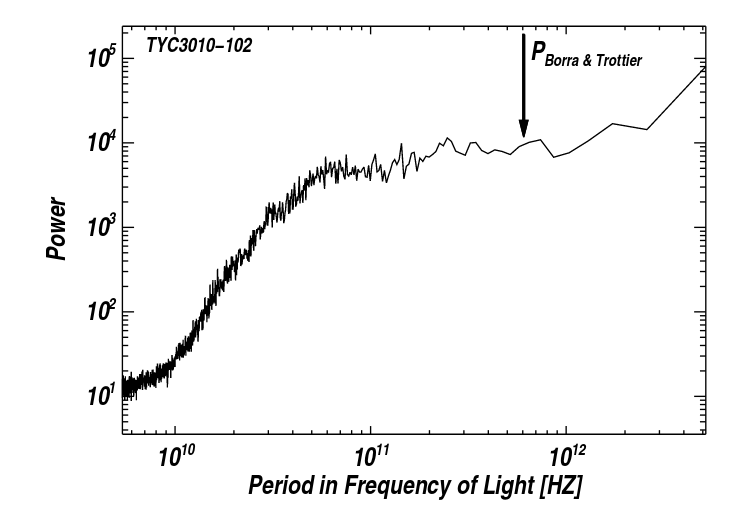
Figure 3 taken from
Isaacson et al. (2018)
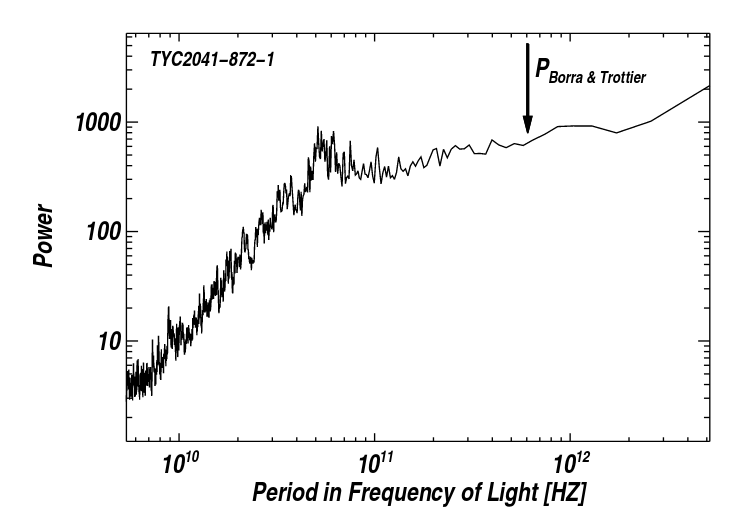
Figure 4 taken from
Isaacson et al. (2018)
Just to be sure that their failure to see the feature was not due to an issue with their Fourier analysis software, Isaacson et al. added an artificial signal into their data, with exactly the period mentioned by Borra and Trottier. They varied the strength of this signal over a wide range, and found that they COULD HAVE detected it if it had an amplitude of a few percent of the continuum.
A more recent paper by Michael Hippke takes a different approach. Is it possible that the signal detected by Borra and Trottier in some Sun-like stars is real, but is present due to natural causes?
Hippke analyzed the spectrum of a star we know very well: the Sun itself! As far as we can tell, there are no creatures modifying the Sun's output in any way, so the spectrum of the Sun should NOT show the presence of this modulation.
However, Hippke's analysis of the solar spectrum shows ... a significant peak at the same frequency, 1.09 x 10⁻¹³ seconds, mentioned by Borra and Trottier.

Figure 1b taken from
Hippke, arXiv 1901.00523 (2019)
Hippke suggests that the natural features due to common atomic absorption lines in the Sun (and similar stars) might just happen, by chance, to occur at rough intervals of around 5 nm, which could give rise to the peak in the power spectrum.
Figure 1d taken from
Hippke, arXiv 1901.00523 (2019)
Copyright © Michael Richmond.
This work is licensed under a Creative Commons License.