 Copyright © Michael Richmond.
This work is licensed under a Creative Commons License.
Copyright © Michael Richmond.
This work is licensed under a Creative Commons License.
Fourier analysis may seem like a completely new and different way to think about repetitive motion, but if you look at it the right way, you may see some common features.
Let's review what we've done so far, so that the ideas are fresh in our minds. We start with some physical situation which corresponds to a mathematical equation. In the case of critically damped harmonic motion, for example, the equation is
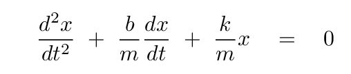
with the additional condition, for critical damping, of
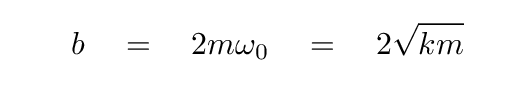
Given this mathematical equation, we can determine a GENERAL form of the equation of motion:
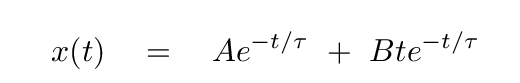
There are two constants of integration in that general equation: A and B. They tell us how to mix the two possible solutions in order to yield the behavior required to match some particular situation; in other words, to match the initial conditions.
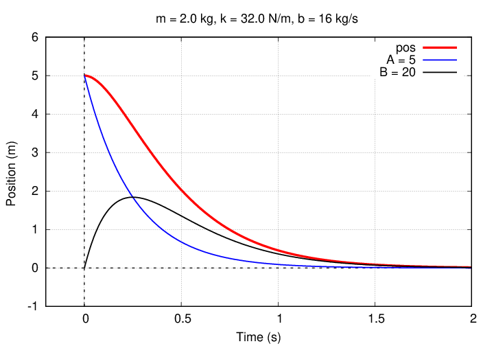
For example, suppose that we are given values of mass, spring constant, and resistive coefficient which yield a time constant of τ = 0.25 s. If the initial conditions are
then it turns out that the proper values for the coefficients of the two terms are A = 5 m and B = 20 m/s. The graph below shows the contribution of each term, as well as the total.
So, to summarize, our approach has been
We will apply these same steps in Fourier analysis.
So, what's the difference? Up to this point, we've considered only motion of a very specific type: governed by a second-order differential equation, objects move in some combination of sinusoidal oscillation and exponential decay. There are plenty of real, physical systems which behave in this way, so it's a fruitful region to consider.
But many other systems do not behave so simply. There are all sorts of crazy motions, far from sinusoids, which occur in nature. It would be nice to have some means to analyze their motion. Fourier methods can be applied to any system with periodic behavior.
Mathematically, this means any system in which some measureable quantity f(t) repeats itself after some period P:
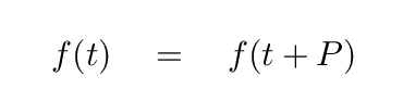
The function may have sharp edges ...
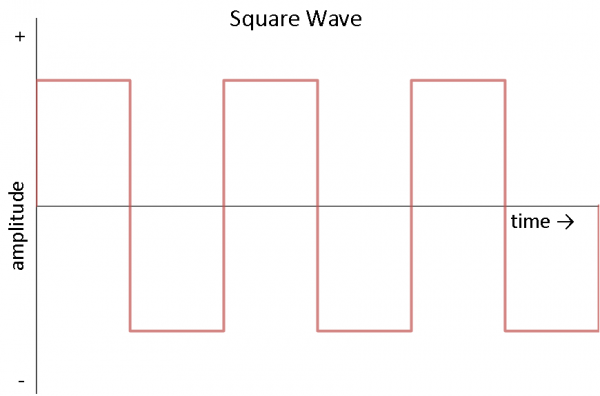
Image courtesy of
Sparkfun tutorials
... or asymmetric rises and dips ...
Light curve of RR Lyr star KIC 8832417,
Figure 1b taken from
Moskalik et al., MNRAS 447, 2348 (2015)
... or it may not be strictly periodic ...
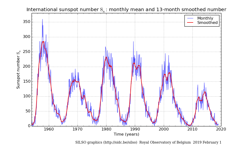
Graph of sunspot numbers courtesy of
SILSO
But we can apply the Fourier technique to all these situations -- and many others. Let's see how.
First, we need a good set of basis functions; these are the functions which we will mix in the proper combination to match the measurements of some particular system. Mathematicians can tell you more about basis functions than I can; for our purposes, it's enough to know that they should
You'll see what the second requirement means in a short time.
  Q:  What would be a good choice for basis functions, which
           can be combined to yield periodic variation?
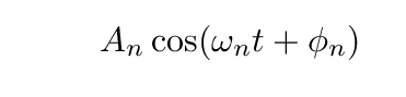
Yes, indeed: sines and cosines. We could choose only cosine functions with a phase offset φ
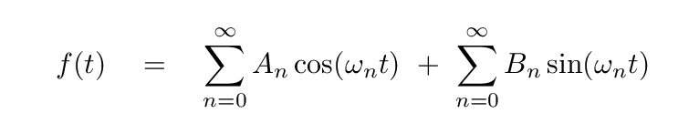
but let's go with a combination of simple sines and cosines:
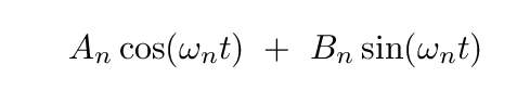
Here, the coefficients An and Bn will depend on the particulars of the measurements we are fitting. The subscript n indicates that we will be adding, not two, not three, but a (possibly) infinite number of sine and cosine terms, each with its own coefficient.
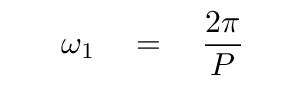
What's the frequency ωn? Well, if the measurements we are fitting repeat over some period P, then it seems logical that one good choice for a frequency would be
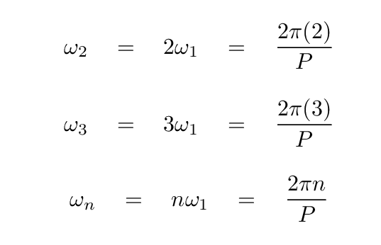
But, it turns out, in order to account for variations on shorter time scales -- which, in practice, means "deviations from a pure sine or cosine wave" -- we need to include a host of other, higher frequencies.
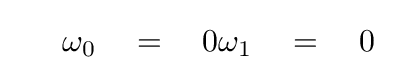
And in order to account for measurements which have a mean value other than zero -- since all pure sines and cosines do vary around zero -- we'll need a term which has a constant value. We can do so if we include
So, we've chosen our basis functions. Good. Our plan is to describe any set of measurements which repeat over a timescale P -- or with a fundamental frequency ω1 = (2π/P) -- as the sum of a series of sines and cosines, using frequencies which are multiples of the fundamental frequency.
The Good News is that, if we figure how to make this work, we will gain a very powerful technique for analyzing a very wide variety of real world measurements.
The Bad News is that we need a possibly infinite number of terms, and that we must compute an appropriate coefficient for each one.
The big challenge is figuring out the value of each coefficient. Our solution will take us down a path leading to long, complicated integrals; it may look scary, but don't worry -- some convenient shortcuts will appear to help us to the goal.
We begin by assuming that is IS possible to represent the periodic function f(t) as
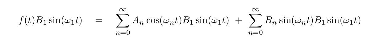
For simplicity's sake, I'm going to pick just one coefficient: B1. I'll go through the process to find the value of B1, but one can apply exactly the same steps to find the value of any other coefficient.
First, we multiply both sides of our equation by the sine (or cosine) term corresponding to the desired coefficient.
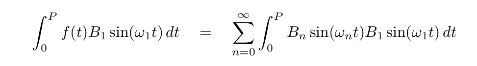
Next, we integrate both sides over one full period P of the function.
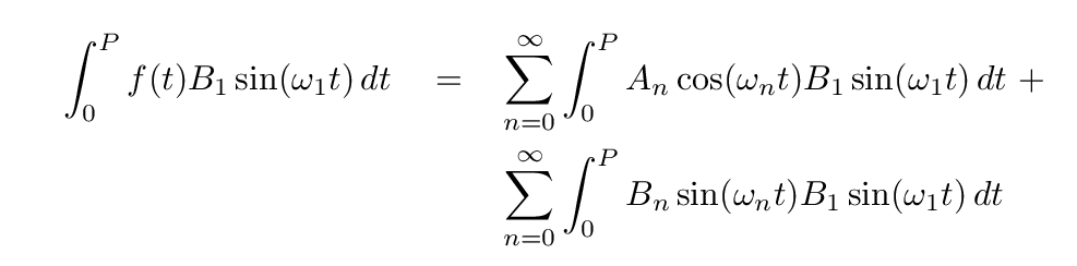
This is the scariest moment. A sum of two infinite series of integrals ... yuck! But as Douglas Adams wrote, Don't Panic.
Instead, look at the first term on the right-hand side. Each term in the sum is an integral over one full period of the product of a cosine and a sine function.

The product of the two shows equal areas above and below the x-axis, which means ....
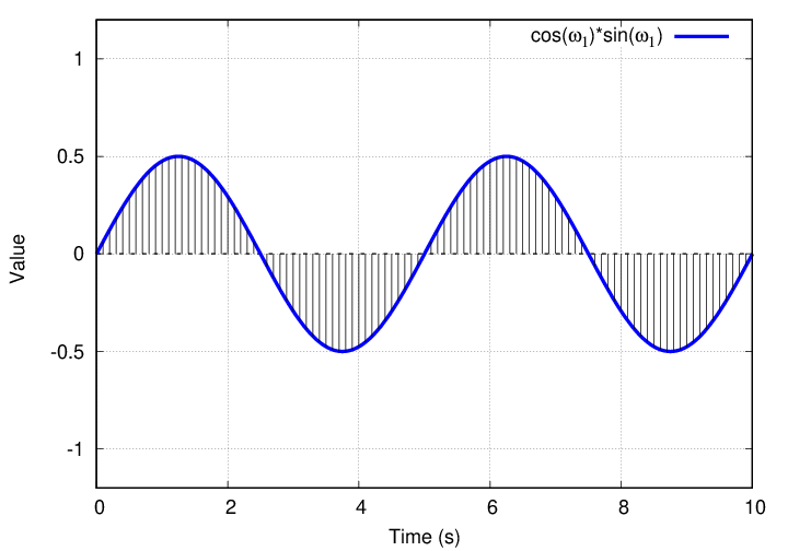
Q: What is the integral of this product over one full period?
Zero.
Suppose we look at the next term in the cosine series; it involves the cosine of a higher frequency ω2.

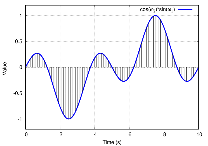
Q: What is the integral of this product over one full period?
The next term in the series involves the cosine of an even higher frequency, ω3.
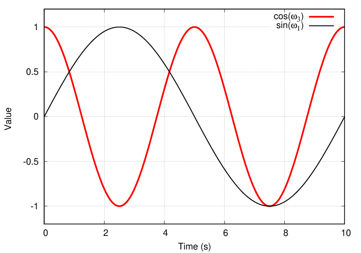
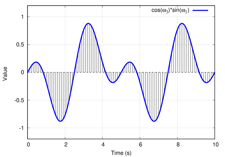
Q: What is the integral of this product over one full period?
Do you sense a pattern here?
It turns out that the integral of the product of ANY cosine function with the sine of ω1 will be exactly zero ... as long as we integrate over one full period. Which we do.
And so, our goal of finding the value of B1 becomes much simpler.
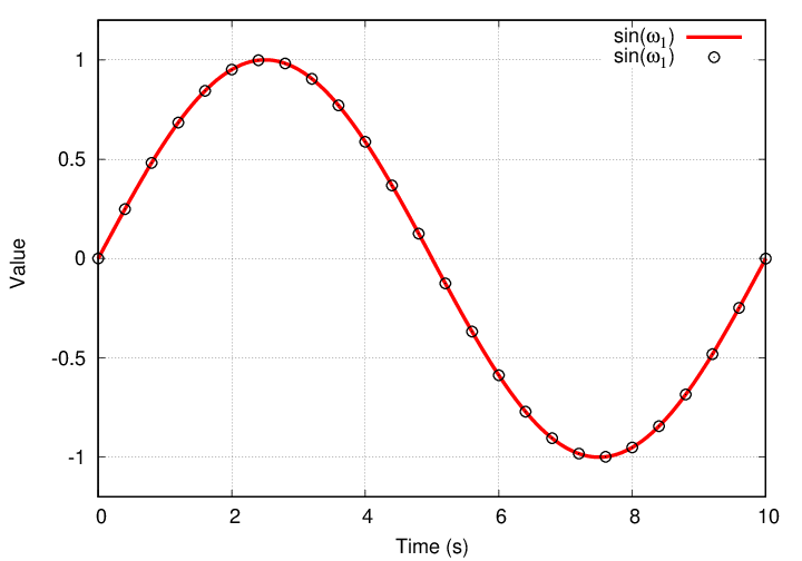
Well, let's see what happens when we multiply a sine function by another sine function. Suppose we look at the fundamental frequency ω1 and the next-highest frequency ω2 ...
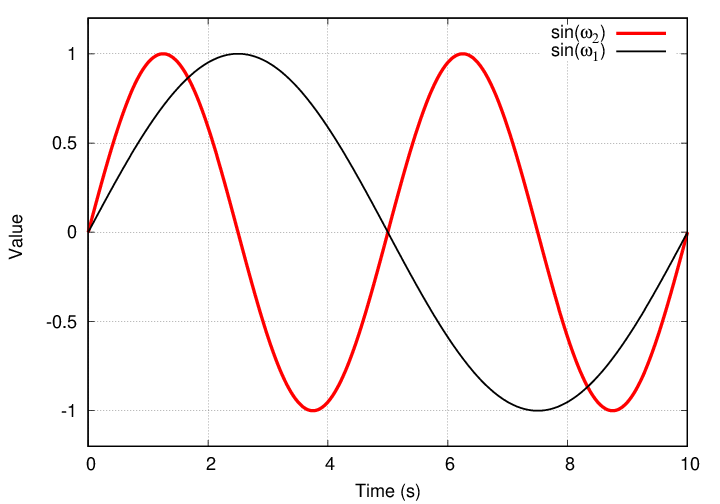
Q: What is the integral of this product over one full period?
Gosh, that yields zero, too.
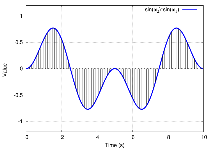
What about a higher frequency ω3?
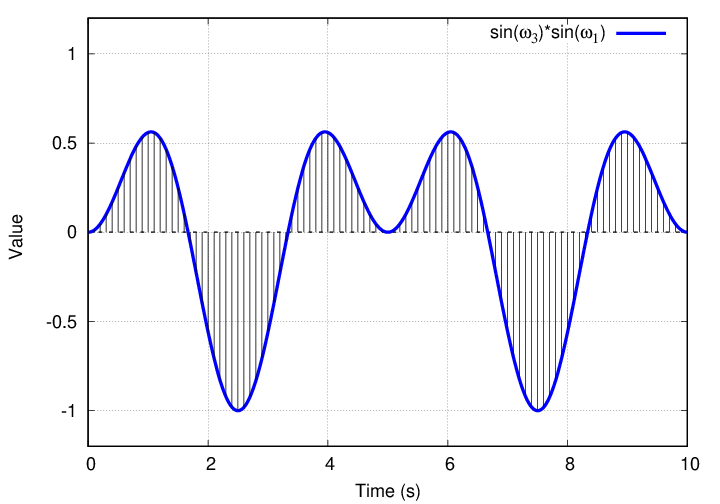
Q: What is the integral of this product over one full period?
Golly. Not only did all the cosine-times-sine terms turn into zero, but it looks like all the sine-times-sine terms yield zero, too.
  Q:  Will EVERY product yield an integral of zero?   Is our whole
            plan doomed?
No, thank goodness. There is exactly one term which yields a non-zero integral. It's the product of sin(ω1) with itself.
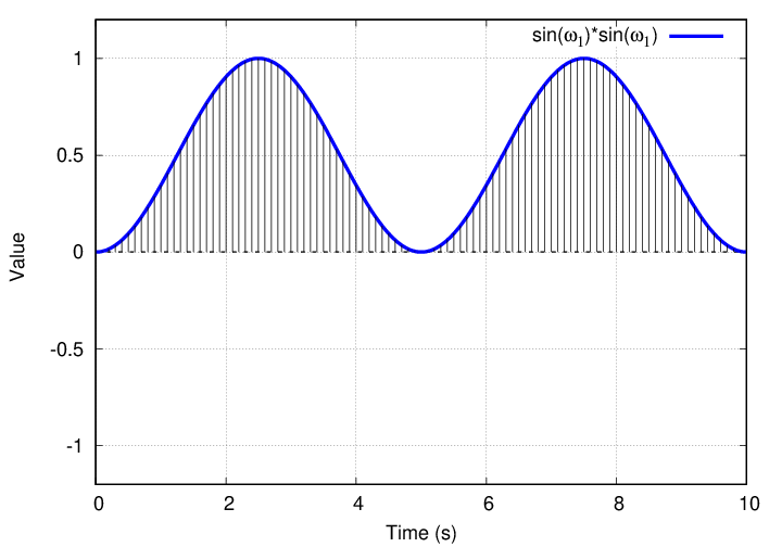
If we can just figure out the value of this integral, then we will be within spitting distance of our goal.
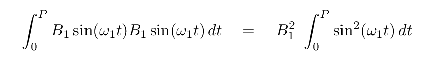
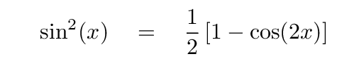
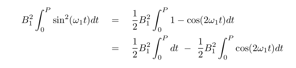
Well, you may recall from your junior-high math class the following trig identity:
If we make this substitution, then our integral turns into
Time for you to do some work.
Q: What is the value of each term on the right-hand side?
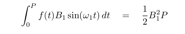
The first integral is equal to P, of course. The second integral isn't so obvious, but it turns out to be zero. So, in the end, the big giant ugly sum of two infinite series
simplifies to
Remember, the reason we started down this path was in order to compute the value of the coefficient B1. Well, we can, at last, do just that.
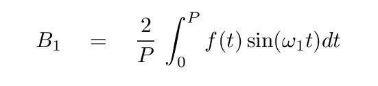
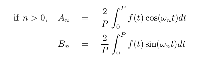
This example centered on the coefficient for the first sine term, B1. But one can use the same approach to find any other coefficient. The general results are -- for any term with n > 0,
The terms with n = 0 are a special case. Following the same procedure, one can derive
Note that the expression for A0 does NOT include a factor of 2.
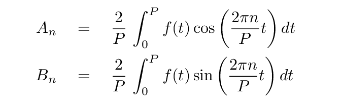
If you prefer to express everything in terms of the period P, one can write these as
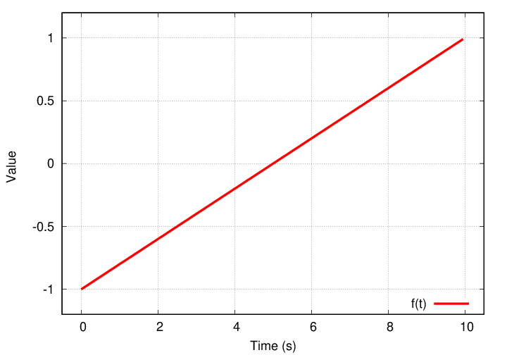
Let's look briefly at the results of this sort of analysis. I'll pick a random periodic function -- how about this one?
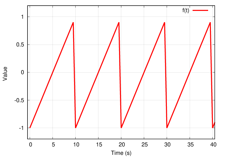
If we look at a single cycle, we see a linear increase from an initial negative value (-1) to a positive value (+1) over a period of 10 seconds.
Applying the method described earlier for finding coefficients, I find that both coefficients of order n = 0 are zero.
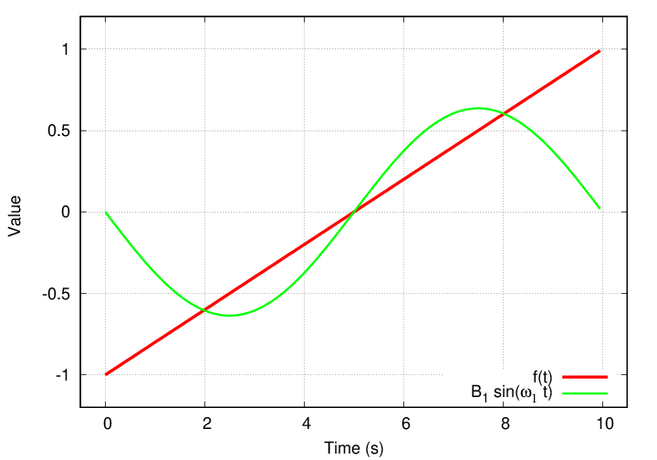
Well, that's not very interesting. If I move on to n = 1, it turns out that the cosine term A1 is again zero, but the sine term is not.
For n = 2, the cosine term A2 is AGAIN zero, but the sine term is non-zero. It's smaller than the first term, though.
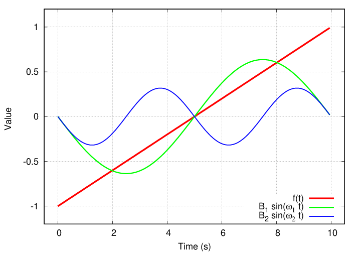
Neither of the individual terms is a very good match to f(t), but if I add them, the sum is a better fit.

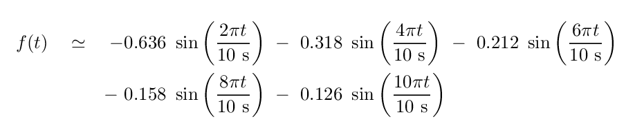
As we continue, we see a pattern: all the cosine terms are zero, and all the sine terms (after n = 0) have negative values which decrease in size.
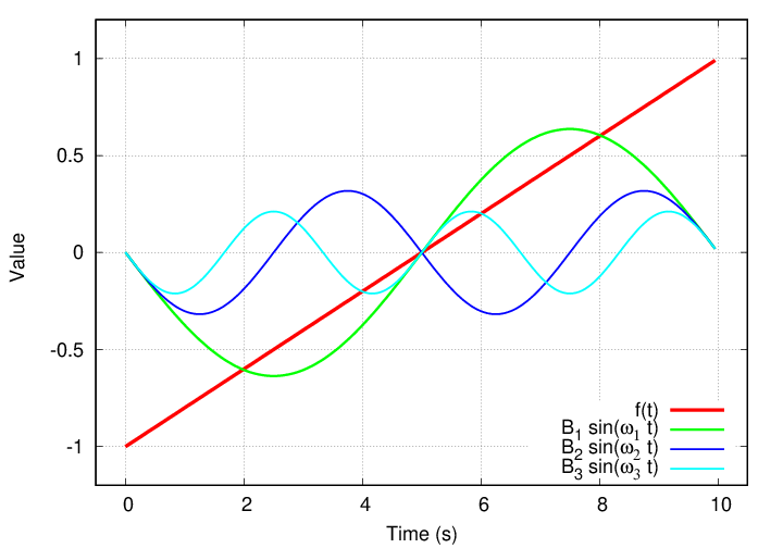
The sum of the sine terms does slowly approach f(t).
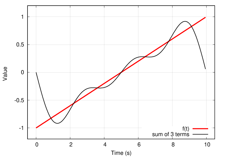
After adding together five terms, the result not terrible ... but not great, either.
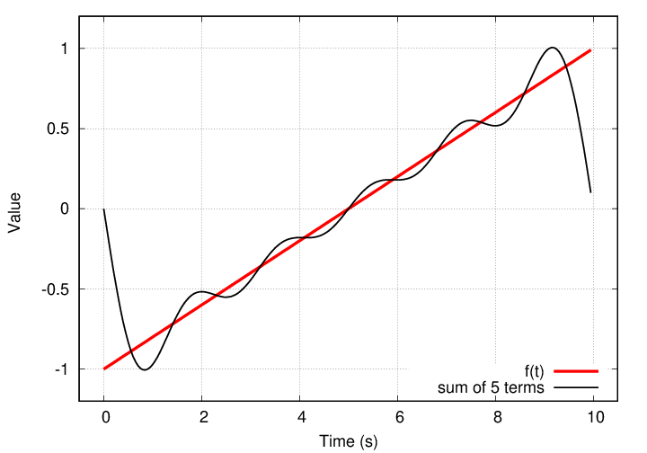
This looks like a case in which it will be necessary to add together MANY terms to match the input function f(t).
Copyright © Michael Richmond.
This work is licensed under a Creative Commons License.