 Copyright © Michael Richmond.
This work is licensed under a Creative Commons License.
Copyright © Michael Richmond.
This work is licensed under a Creative Commons License.
In many, many situations that involve oscillating systems, a common factor pops up. Usually denoted by the letter Q, and sometimes called the quality factor, this quantity has several different meanings. We'll only discuss a few of them here.
It's not only in mechanical systems, such as pendula or shock absorbers, that this "Q" factor appears. The same equations govern a number of electronic systems, such as the simple series RLC circuit shown below:

Image courtesy of
Wikipedia
Let's begin with a damped harmonic oscillator, without any driving force. We'll add that complication later.
In this case, the differential equation is
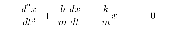
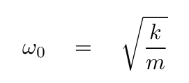
We've solved this differential equation; the solution is a combination of oscillations and exponential decay

where the natural, or un-damped, frequency of oscillation is
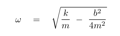
the damped frequency of oscillation is
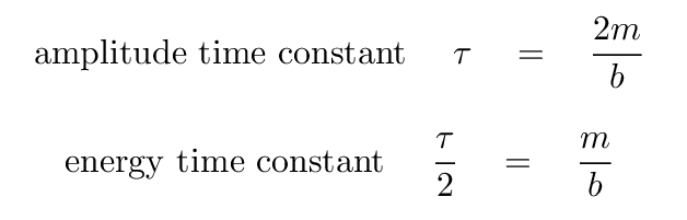
and the time constant τ of the decay depends on the mass and coefficient of the resistive force.

What about the ENERGY of this system?
  Q:  How does potential energy depend upon (maximum) displacement?

  Q:  How does kinetic energy depend upon (maximum) velocity?
Right. The energy depends on the SQUARE of the displacement, and on the SQUARE of the velocity. For example, the spring potential energy at any time is

  Q:  What is the time constant associated with the decay of
             spring potential energy?
In this case, the decay is faster than that of amplitude. We could define a new "energy time constant", if we wished.
So, "how long does it take for amplitude or energy to decay" is one timescale associated with this system. But it's not the only one.
We can also ask another sort of time-related questions:
   Q:  How long does it take for the system to oscillate
               by one full cycle?


   Q:  How long does it take for the system to oscillate
               by one radian?

You may be wondering why the equations above use the natural angular frequency ω0 instead of the damped frequency ω. One reason is "this is the convention," but that's not very satisfying. Another reason is that most of the systems for which we will compute "Q" are under-damped, so the two angular frequencies are very, very similar ... and the natural frequency is much easier to compute.
This gives us four time-related quantities that we could compare.
        decay times                oscillation times
----------------------------------------------------------
         amplitude                    one cycle

         energy                       one radian
----------------------------------------------------------
The choice that most textbooks and analyses make is to compare the decay time of ENERGY to the time it takes the system to move by one RADIAN.
                     decay time for energy
     Compare    ---------------------------------
                   time to oscillate one radian


     Q:  Write down an expression for this ratio.
                 Try to write it in terms of the mass m
                 and resistive force coefficient b.
You should end up with a quantity known as Q, the quality factor. Note that Q is a pure number, with no units.

Why is it called the "quality factor"? Well, it clearly describes something important about an oscillating system: something related to the number of cycles it takes for the motion to die down.
I guess that people who work with oscillating systems tend to like the ones which keep going for many cycles.
So, one thing that Q tells us is something about the decay of an oscillating system.
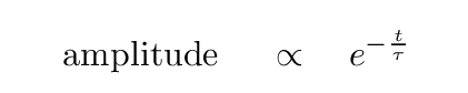
You may be familiar with the use of the time constant τ. In the time τ, the amplitude of motion decreases to 1/e of its original value.

But how much does the amplitude decrease in just one cycle? In other words, how much does the amplitude decrease during a time P?

Well, if you start with the basic exponential decay
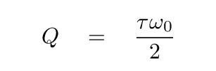
and if you remember that one way to write Q is
then you should be able to write an expression for the factor by which the amplitude decreases during a single period.
Q: By what factor does the amplitude decrease in one cycle?
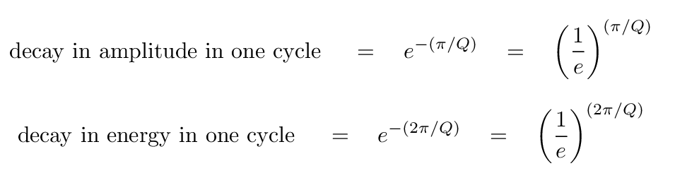
Hmmm. If we know the factor is f for just one cycle, then we know that after TWO cycles, the decrease will be f2, and after THREE cycles, the decrease will be f3, and after N cycles, the decrease will be fN.
  Q:  How many cycles will it take for the amplitude to decrease
             to a value of (1/e) of its original value?
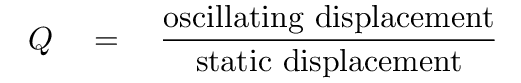
Another aspect of the "Q factor" can be seen if we compare the response of a system to static and oscillating forces.
Consider a standard spring of force constant k, from which we hang a mass m. We let the system come to rest at an equilibrium, marked by the dashed line in the figure below. Then, we pull on the mass with a STATIC force Fmax.
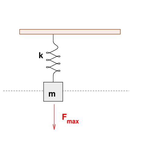
Q: How large is the resulting displacement of the mass?

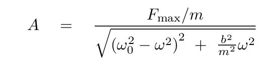
Now, suppose that we pull down again, but this time with a VARYING force, F(t) = Fmax eiωt. How big is the displacement of the mass now?
"Aha!" you say. "That depends on the frequency ω of the driving force, and how it compares to the natural frequency ω0 of the spring and mass."
Right you are.
  Q:  Suppose that the driving frequency is exactly equal to the
              natural frequency of the system.
              What will the amplitude of motion be?
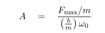
Now, if you recall that one way to write Q is

and if you recall the definition of ω0, you should be able to write the amplitude in a form which includes Q.
  Q:  How can you write the amplitude at resonance in a way
              that includes Q, and is easy to compare to the
              static displacement?
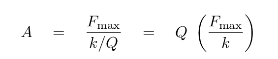
And so we see that the amplitude of motion for the forced, oscillating system at resonance is exactly Q times the displacement by a static force of the same size.
As you know, the amplitude of a forced harmonic oscillator depends on a number of factors. A general result is that the amplitude is large when the driving frequency is close to the natural frequency of the undamped system.

  Q:  In the figure above, what is the natural frequency ω0?


  Q:  Compute the value of "Q" for each choice of b.
It's clear that the value of Q is related to the shape of this amplitude graph.
But let's put the relationship on a quantitative scale. It will take a while, but the result in the end will be worth it.
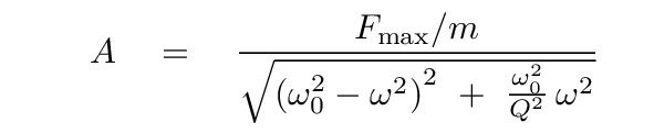
First, we write the amplitude as a function of driving frequency in a slightly different manner, so that "Q" appears in it.
Now, we are going to switch from dealing with the amplitude of motion to the power dissipated in a driving oscillating system. What does that mean? The system has a resistive force, remember? That means that as the system moves, the resistive force does negative work, and so that system loses energy. The only reason it keeps oscillating is because we are driving it!
In other words, the power dissipated is the power we must supply to the driving force to keep the system going.
Now, the power dissipated by the system can be described as energy lost over time. We know how the energy of a harmonic oscillator depends on the amplitude.
Energy of oscillating system ∝ (amplitude)2
And it turns out that the same is true for the power dissipated. So, we can write that the power lost by this system goes like the amplitude squared, or
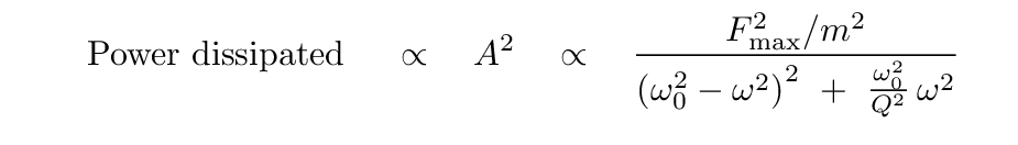
Let's make a graph showing the power dissipated as a function of the driving frequency. It will have a peak close(*) to the natural frequency of the system, and some width around that peak.
(*) yes, the maximum dissipated power occurs at a slightly lower frequency than ω0, but for most cases of interest, this difference is very small. Assuming the peak is exactly at the natural frequency will simplify some of the expressions which follow, so let's do that.

It turns out that Q will be related to the ratio of these differences, Δω, to the peak frequency ω0.
Q: Estimate the fractional width of the peak in the graph above.
Let's see how to find that relationship.
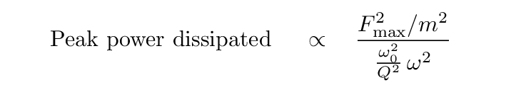
Start with the equation for power dissipated.
Q: What is the power dissipated at resonance?
Right.
Now, if we shift the driving frequency away from resonance, just far enough that the power dissipated has HALF its peak value, then the denominator of the expression must be exactly TWICE the size of the denominator at the peak: dividing by something twice as big will yield power which is half the size. That means that at a half-power point,

Simplifying a bit,

Now, here we make an approximation. Most of the time, when we discuss the properties of oscillating systems, the systems will be relatively "high-quality" oscillators. That means that the Q factor will be high, and so the dissipated power will span only a narrow range of frequencies. In such cases, the driving frequency will be close to the resonant frequency, ω ~ ω0, and so the sum of (ω + ω0) is approximately twice the resonant frequency.
With that approximation, we can write
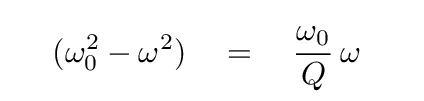
  Q:  Write an equation which has the difference between driving
            and resonant frequencies on the left,
            and everything else on the right.
You should end up with something like this (again, recalling that ω ~ ω0):
This looks useful. Go back to the graph of power dissipated as a function of driving frequency.
The fractional width of the dissipated power is (basically) the reciprocal of Q.
This width of frequencies over which the system dissipates (or perhaps produces) power is sometimes called the bandwidth of the system.
There are a myriad applications of systems in which the creation of a narrow bandwidth is a key feature. One of my favorites is
the humble radio tuner.
  Q:  Suppose that you are designing a radio tuner which should
             be able to distinguish two radio stations which
             are at

                 station A:   93.3  MHz

                 station B:   93.7  MHz


             What value of Q must your electronics produce?
Copyright © Michael Richmond.
This work is licensed under a Creative Commons License.