 Copyright © Michael Richmond.
This work is licensed under a Creative Commons License.
Copyright © Michael Richmond.
This work is licensed under a Creative Commons License.
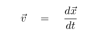
Recall from our earlier discussion the kinematic quantities -- position, velocity, and acceleration:
| x | position | meters (m) |
| v | velocity | meters per second (m/s) |
| a | acceleration | meters per second per second (m/s2) |
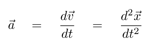
There are mathematical relationships between these quantities:
We can use these relationships to find out what happens if the acceleration is constant. It's a special case, sure, but here on Earth, it's a very, very common special case.
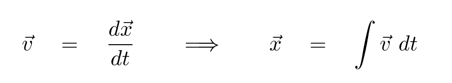
Let's begin by doing a little calculus. We can turn the connection between velocity and acceleration inside out to find out what a constant acceleration means for velocity:
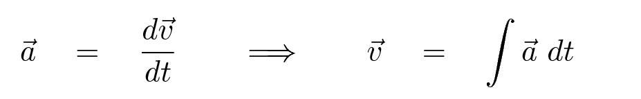
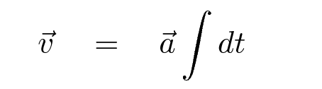
But if the acceleration is constant, we can take it out of the integral.
Q: Can you do this integral?
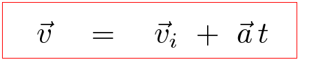
Right. We end up with a linear function of time. The constant of integration can be interpreted as the initial velocity of the object. One way to write the result is:
What about position? Can we figure out how it changes with time under constant acceleration? Sure -- just do the same sort of analysis.
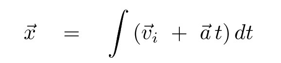
If the acceleration is constant, this becomes
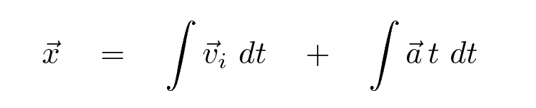
We can split up the integral into two pieces.
Q: Can you do this integral?
Right. There will be two constants of integration in this case, but we can collect them into a single term, which we can interpret as the initial position of the object. One way to write the result is:
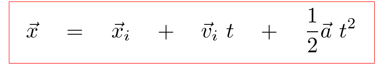
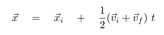
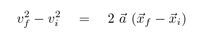
We've derived two very useful equations relating the kinematic quantities. With a little algebra, one can derive additional equations by re-arranging the terms and solving for various quantities. One often finds two of these re-arranged equations listed in textbooks, simply because they frequently come in handy:
Copyright © Michael Richmond.
This work is licensed under a Creative Commons License.