A cart rolling down a track

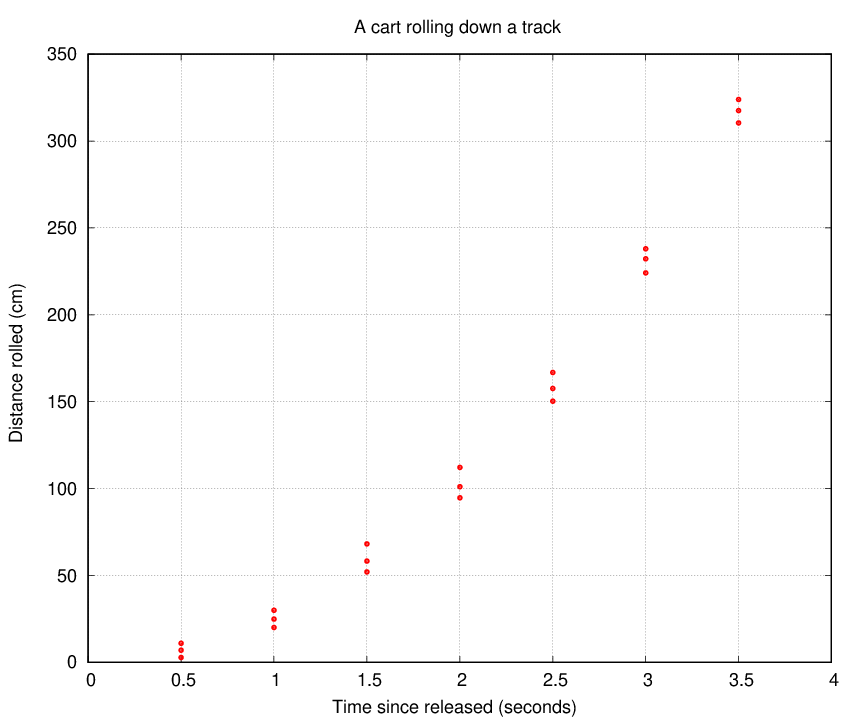
I raised one end of a long track slightly, so that it was tilted from left to right. Then I placed a small cart on the track near the top, released it, and measured how far it rolled during several intervals. Here is a table of my measurements.



# Time   Trial_1    Trial_2     Trial_3    Mean_pos   Stdev_pos   
# (s)     (cm)       (cm)       (cm)       (cm)        (cm)
#------------------------------------------------------------------

0.5        7.0        2.8       11.0                                

1.0       20.1       30.0       24.9                             

1.5       68.2       52.1       58.3                             

2.0      112.2      101.1       94.7                             

2.5      150.3      166.8      157.6                            

3.0      232.2      224.1      238.0                             

3.5      323.9      317.5      310.4                            
#------------------------------------------------------------------

A graph showing position as a function of time has a curved shape:



# Time   Trial_1    Trial_2     Trial_3    Mean_pos   Stdev_pos   
# (s)     (cm)       (cm)       (cm)       (cm)        (cm)
#------------------------------------------------------------------

0.5        7.0        2.8       11.0                                

1.0       20.1       30.0       24.9                             

1.5       68.2       52.1       58.3                             

2.0      112.2      101.1       94.7                             

2.5      150.3      166.8      157.6                            

3.0      232.2      224.1      238.0                             

3.5      323.9      317.5      310.4                            
#------------------------------------------------------------------

Your first job is to turn the 3 measurements for each time value into a single value with an uncertainty. Therefore, your team should compute the MEAN and STANDARD DEVIATION of each set of positions.

What are they? Well, the mean is the same as the average.

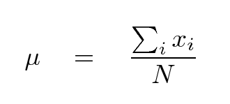
For example, the mean position after t = 0.5 seconds is


                     7.0  +  2.8  +  11.0
        mean   =   -------------------------  =  6.93  cm
                             3

The standard deviation is one way (not the only way) to represent the scatter of a bunch of numbers around their average value. Mathematically, one can compute it as follows:

The standard deviation of the position after t = 0.5 seconds is


                                                                            0.5
                 [  (7.0 - 6.93)^2  +  (2.8 - 6.93)^2  +  (11.0 - 6.93)^2  ]
      stdev    = [  ------------------------------------------------------ ]
                 [                      2                                  ]

               =   4.10  cm

You can find more examples for these calculations in my guide to uncertainties.

Here are my results:


# Time   Trial_1    Trial_2     Trial_3    Avg_pos    Stdev_pos   
# (s)     (cm)       (cm)       (cm)       (cm)        (cm)
#
0.5        7.0        2.8       11.0        6.93       4.10
1.0       20.1       30.0       24.9       25.00       4.95
1.5       68.2       52.1       58.3       59.53       8.12
2.0      112.2      101.1       94.7      102.67       8.85
2.5      150.3      166.8      157.6      158.23       8.27
3.0      232.2      224.1      238.0      231.43       6.98
3.5      323.9      317.5      310.4      317.27       6.75

Computing average velocities, and their uncertainties

Each group must complete the following calculations. I recommend splitting the work up, and (if you have enough people) assigning two people to each calculation, so they can check each other.

Using consecutive measurements, figure out the average velocity between each pair of positions. The average time for this average velocity is the half-way point in time between the measurements. You should end up with 6 values for average velocity and the time for each. Make a neat table showing the average velocities and the time associated with each.

Determine an uncertainty in each average velocity. To do this, use the method of extremes:



               t1  =  1.5 s     x1    =    32.0  +/-  3.0  cm
               t2  =  2.0 s     x2    =    63.0  +/-  4.0  cm

                                    (63.0 - 32.0) cm
               avg velocity   =   ---------------------  =   62.0 cm/s
                                    (2.0  - 1.5)  s



                                  (63.0 + 4.0) - (32.0 - 3.0)  cm
               max velocity   =  --------------------------------- =  76.0 cm/s
                                        (2.0  - 1.5) s

                                  (63.0 - 4.0) - (32.0 + 3.0)  cm
               min velocity   =  --------------------------------- =  48.0 cm/s
                                        (2.0  - 1.5) s



               uncert in avg velocity  =  one half of (max - min)

                                       =   0.5 * (76.0 - 48.0) cm/s  

                                       =   14.0 cm/s


               avg velocity  =  62.0 +/- 14.0  cm/s

When you have finished, call one of the instructors over so we can check that everything looks correct.

Here are my results:


# Time     Avg_vel   uncer_vel
# (s)      (cm/s)     (cm/s)
#
0.75       36.14      18.10    
1.25       69.06      26.14
1.75       86.28      33.94
2.25      111.12      34.24
2.75      146.40      30.50
3.25      171.68      27.46

Use a graph to determine the average acceleration of the cart

Great! We now have estimates for the average velocity of the cart at different times as it rolled down the track. You should see that the velocity increases with time. In other words, the cart was accelerating.

Let's try to compute the acceleration of the cart by making a graph which shows the velocity as a function of time.

Make a graph of your values, placing average velocity on the y-axis and average time on the x-axis. Be sure that your graph has proper labels on each axis.

Use the uncertainty in each value of average velocity to draw a vertical errorbar around each symbol.

Draw lines on this graph in order to estimate the acceleration of the cart. Use this guide to determine the uncertainty in the slope (and, thus, the uncertainty in the acceleration).

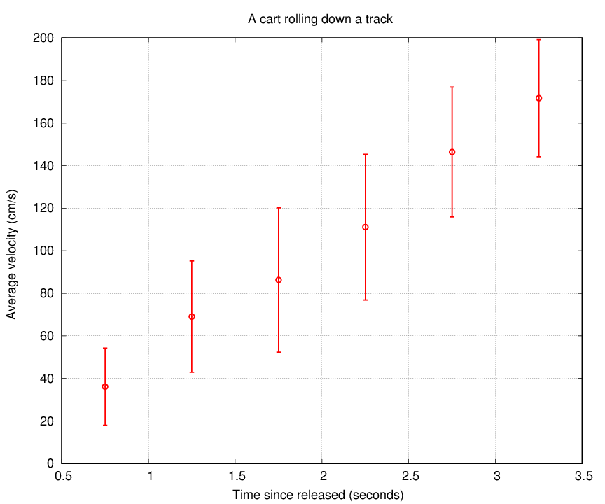
There's quite a wide range of values for the slope which are consistent with the data.



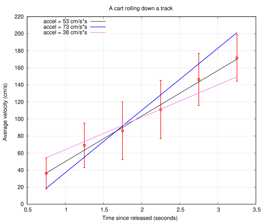
  Q:  How might you write the acceleration of the cart?

If you drop a cart, it falls through the air with an acceleration which is about g = 980 cm/s². How does that compare to the acceleration of my cart as it rolled down a ramp? Be quantitative!