Conservation of Energy as a spring oscillates

You should prepare for this experiment before class.

Prelab questions

The goals

Find the effective mass of the spring
Find the spring constant of the spring
Find the "phase difference" during oscillation between
1. force and displacement
2. force and acceleration
3. force and velocity
4. kinetic energy and spring potential energy
Check to see if total energy is constant over several full cycles
Check to see if total energy is constant over a period of five or ten minutes

Setting up the experiment

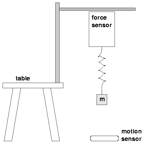
Set the slide switch on the force probe to 10 N. Place the motion sensor on the floor. Attach the force sensor to CH 1, and the motion sensor to Dig/Sonic 1.
Open the experiment Mechanical Energy.
Calibrate the force sensor.
Orient the spring with the wide end up, and tape blocks to the mass hanger for a total of about 250 g. The mass should be about 15 or 20 cm below the bench top at equilibrium. Zero the sensors with the block at rest.
Check your set-up by lifting the mass straight up about 5 cm and releasing it. Avoid side-to-side motion. What do you expect to see for position as a function of time? Collect data; do you see what you expected? If not, adjust the sensors until you get what you expect.
You should see the position oscillate around 0 meters (to within about +/- 0.001 m), and the force oscillate around 0 Newtons (to within about +/- 0.0003 N). Look carefully; if the centers of oscillation aren't zero, you may have to adjust the readings manually to force them to zero.
Adjust to zero manually: Return the system to equilibrium and zero all sensors. Collect data with the system at rest. Use Analyze:Statistics to determine the average position of the mass. Click on the oval Labpro icon to bring up the Sensors Window, and click on the motion sensor. On the pop-up menu, click Set Offset. A box will pop up with an initial value of the offset. Subtract the average position from the offset and enter this difference as the new offset, then click OK. (E.g. if the average position is 0.0123 and the initial offset is -0.612345, the new offset is -0.624645.) Collect data again and the position should have an average very close to zero. Close the Sensors window. Each time you zero the motion detector you will need to repeat this.

Use Analyze Data Examine to look at the highest and lowest distance the mass reaches. If these two extremes are not the same size, make appropriate adjustments and take new data. If sometimes helps to wait one minute after starting the block in motion before you collect data.

Be absolutely certain that you have the equipment properly zeroed or your results will be bogus!

Collecting a first dataset

Start the mass moving and let it oscillate for about one minute; higher order vibrations will damp out during this time, leaving very smooth, simple, harmonic motion. Press Collect to gather data. You should see nice smooth sine wave shapes for position and velocity. Before you go any further, ask an instructor to verify that your data is good enough.

Analysis over a few cycles

You can (and should) print out several graphs to illustrate your report. If you want to plot more than one measurement on the vertical axis, click the name, click More on the pop up menu, and check the boxes for the additional quantities you wish to plot.

Compare the Force and Position graphs, and give a verbal description of their relation. Are force and displacement "exactly in phase", "exactly out of phase", or something else? Explain.
Compare the Force and Acceleration graphs, and give a verbal description of their relation. Are force and acceleration "exactly in phase", "exactly out of phase", or something else? Explain.
Compare the Force and Velocity graphs, and give a verbal description of their relation. Are force and velocity "exactly in phase", "exactly out of phase", or something else? Explain.
Find the spring constant k by making a graph of one particular quantity versus another. Make a linear fit to the graph and record the fitted parameters, which will have names like "y" and "x". Re-write the equation so that the variables have their proper names and units (hint: the left-hand side should be "Force", in Newtons).
Find the effective mass m of the spring by making a graph of one particular quantity versus another. Make a linear fit to the graph and record the fitted parameters, which will have names like "y" and "x". Re-write the equation so that the variables have their proper names and units (hint: the left-hand side should again be "Force", in Newtons).
Create formulas within LabPro for kinetic energy (KE) and potential energy (U).

To create a new column for kinetic energy, go to Data: New Calculated Columns and enter values for the name (e.g. Kinetic Energy), short name (e.g. KE), and units (J). In the Equation box, enter the formula for kinetic energy. You should know the effective mass from part 8 (suppose you found 0.999 kg), and can get the velocity from the Variables pull down menu. The equation should look something like
```
           0.5 * 0.999 * "velocity"^2
```
In a similar fashion, define the potential energy, U, and the total mechanical energy, E = KE + U. If you need to change a definition, select the column from Data:Column Options and an editing widow will appear.
Make graphs that allow you to discuss conservation of energy. Examples of graphs might be any one of the energies versus time (or position, or velocity, or acceleration), one energy versus another energy, etc. You need to try different graphs and decide what they tell you about energy conservation.
Is energy conserved during your measurements? There are two ways to answer this question:
1. what is the "peak-to-peak" change in the total energy, expressed as a fraction of the average total energy? You should be able to state something like "total energy bounces around its mean by around +/- 2 percent."
2. what is the secular change in the average total energy during the period you measured? You might compare the average energy during the first second of data to the average energy during the final second of measurements.

Analysis over a very long period

You ought to find that total mechanical energy is almost exactly the same over a few cycles of oscillation. But what if we monitor the system over many, many cycles? Change the Experiment->Data Collection parameters so that you measure 10 samples per second over a period of 500 seconds (yes, that's about 9 minutes).

Reset the system to equilibrium and re-zero the sensors
Pull the weight down about 5 cm and release it carefully. Wait about one minute to let the wiggles dissipate
Collect measurements over the long period
While you are waiting for this to finish, you might perform calculations for the previous portions of the experiment, or start writing your report.
Look at (and print) a graph of Total Energy versus Time. Is energy conserved over this long period?
What is the "half-life" of energy? That is, how long does it take for the total energy to decay to half its original value?
Fit the Total Energy versus Time graph with an exponential curve. Record the parameters displayed by LabPro. Re-write the equation so that it looks like this:

where t is the time in seconds and E0 the initial energy of the system. What is the time constant tau of the system?
How much energy would be left if the spring continued to oscillate for one hour?

For more information

You can save your data file(s) and analyze them outside of class by downloading a demo version of Logger Pro or by grabbing a copy of LabPro from the SVPHY01 server in Science Bldg Zone.