
When analyzing measurements in any branch of science, one often wishes to compare the measurements to some sort of model with adjustable parameters. For example, measurements of the potential energy of a metal spring, when it is stretched or compressed to various lengths, yield the following results:
        dist(cm)       PE(Joules)
    ----------------------------------
          9             10.0
         10              6.6
         11              3.2
         12              1.0
         13              1.4
         14              2.8
         15              7.2
         16              9.8
    ----------------------------------
A graph of potential energy as a function of spring length shows a relationship that looks rather quadratic.
We might therefore create a model for this relationship. Using the variable x to stand for the length of the spring, our model might be

where a, b, and c are three model parameters. In order to make the model match the measurements, we need to find just the right values of these parameters, those which will, for any chosen length of the spring, cause the model to predict potential energies which are nearly equal to the measured potential energies. In other words, we would like to find the "best-fitting values" of these model parameters.
If one has chosen a model properly, this will often be possible. In this particular example, if we choose
then our model does a fairly good job of reproducing the data.

But how can we figure out the values of those parameters?
The goal of this document is to explain how one might set up a mathematical procedure which leads to the "best-fitting" values of a set of model parameters. One can, of course, simply call upon some pre-existing function within a mathematical library, or run some sophisticated software package which performs such tasks automatically. If one simply wishes to know the answer for some particular problem, that's fine; stop reading and simply run the code. But if one wants to look behind the curtain a bit, and investigate some of the inner workings of those black boxes, then read on.
The dataset I'll use throughout this document is a set of measurements of the position of a relatively nearby star over the course of roughly one year.

The next section of the text will explain why the motion of the star has a somewhat lopsided corkscrew-like shape, and provide a bit of background for the model equations that we will use to fit the measurements. Those who simply want to see the math behind the model-fitting may choose to skip it.
In this section, I'll discuss the basic reason for the motion of a star in the sky over a period of several years, which may help to explain the equations which will appear in the following sections. If you only care about the algorithmic details of fitting a model to data, you might skip this section.
Let's begin by imagining a view of the Solar System from far above the plane of the planetary orbits. A view of the inner planets would look something like this:

Image created with the excellent
Celestia software .
Click on the image to show two years' worth of motion.
The Earth's orbit is highlighted in red. Over the course of one year, the Earth moves all the way around that nearly circular path. If you click on the image, you can watch a short movie showing the Earth's motion from above.
That motion of the Earth around the Sun affects our view of nearby stars. In the diagram below, consider pictures that we take of the nearby target star over the course of a year.

During the month of January, when the Earth is on one side of its orbit, the target star will appear close to star "W". But six months later, in July, when the Earth has moved to the other side of its orbit, the target star will appear close to the star labelled "Z". Over the course of a full year, the target star will appear to move in a small, nearly circular ellipse relative to more distant stars.

This small shift of nearby stars is called parallax.
The Gaia spacecraft has measured the parallax motions for billions of stars very carefully over several years. Scientists at the European Space Agency have made a movie showing an exaggerated version of these little ellipses which they have observed.
Now, what happens if we look at stars which aren't directly above the plane of the Earth's orbit, but instead lie off to the side? (Once again, click on the image to see a movie showing the motion of the Earth).

Image created with the excellent
Celestia software .
Click on the image to show two years' worth of motion.
In this case, we'll still see nearby stars appear to shift back and forth over the course of a year, but the motion will be restricted into one dimension.

In the general case of a nearby star located at some arbitrary location in space, neither directly above, nor directly in, the plane of the Earth's orbit, the parallax motion will appear as a tilted circle -- in other words, as an ellipse.

The exact shape of this ellipse will depend on the particular location of the star, relative to the plane of the Earth's orbit.
But wait -- we've only told half the story so far. It's true that the Earth's orbital motion around the Sun causes nearby stars to appear to move in small ellipses. But this periodic wobble is combined with a second type of motion. The Sun and all the other stars in the Milky Way Galaxy are flying around the center of the Galaxy. Even though most are moving in the same general direction, and with very roughly similar speeds, each star has its own particular velocity. That means that some stars are catching up to the Sun and others are falling behind. Over the course of many centuries or millenia, these small differences in motion cause each star to drift slowly across our sky. Astronomers call these gradual drifts proper motion.
Now, if we only account for proper motion, and ignore the periodic cycles due to parallax for a moment, we would expect stars to move in perfectly straight lines across the sky.

When we combine the effects of parallax and proper motion, we find that a star's path resembles a helix or corkscrew.

For stars with large proper motions, the corkscrew becomes stretched out into a slightly skewed sinusoid.

If we wish to create a model of this motion, including the effects of both parallax and proper motion, we need to account for the following factors:
Some of these quantities -- such as the obliquity of the ecliptic -- have been measured very carefully and can simply be taken from a catalog or almanac. Others -- such as the ecliptic longitude -- are based on similarly well-known quantities, and can be calculated precisely for any given date of observation. It will turn out that the proper motion values, μα and μδ, will be two of the parameters which we will vary as we attempt to fit a mathematical model to a set of observations.
In this section, we'll go through a bit of mathematical manipulation in order to write a pair of equations which allow us to compare directly the observations of the star's motion to a model. The goal of our work will be to put those equations into a special form, which has
In this example, the model ends up in a particularly felicitous form: each of the parameters we wish to fit appears just once on the right-hand side, and each appears to the first power. In other words, our model will feature LINEAR factors of each parameter to be fit.
Our model for the motion of the star will predict its position in Right Ascension, α, and Declination, δ, at any given time. More precisely, it will predict the amount by which its position has changed from some starting point α0 and δ0 at some given starting time t0. In other words, our model will predict the changes in RA and Dec over time, (α - α0) and (δ - δ0).
These changes depend upon two effects. First, the motion of the Earth around the Sun, which causes us to see a star from slightly different viewpoints over the course of a year. We can refer to these periodic shifts back and forth as the parallactic shift. Second, the relative motion of the Sun and the target star as they both move through the Milky Way Galaxy causes the star to appear to creep across the sky very slowly; this is called the proper motion of the star.
Although the parallactic shift is due to the Earth's motion around the Sun, computing its effects are somewhat easier if one considers the apparent motion of the Sun around the sky. The important factor here is the ecliptic longitude of the Sun, λ. In order to predict the apparent position of a star on some given date t, we need to calculate this quantity for that date. Following the formulae provided in the US Naval Observatory's Astronomical Almanac, we can compute λ in a relatively simple three-step procedure. First, we compute the Sun's mean longitude L for some given time t

where L0 is the mean longitude at the starting time t0.
Next, we compute the Sun's mean anomaly g

where g0 is the mean anomaly at the starting time.
We can now calculate the Sun's ecliptic longitude λ

Once we have a value for the Sun's ecliptic longitude, we can go on to make our prediction for the position of a star. Let's first write down an expression for the Right Ascension.

The terms appearing in this equation are
Strictly speaking, this equation is real mess: the Right Ascension α at the time of interest t appears on BOTH the left-hand and right-hand sides of the equation. Yuck. However, as long as we restrict ourselves to the motions of stars over relatively short timescales -- say, a decade or two -- we can make a handy approximation. Over these timescales, all stars will only move a very small fraction of a single degree. Note that the RA on the right-hand side always appears inside a "sine" or "cosine" expression. We can make very good assumptions that

and therefore replace the changing, actual Right Ascension α on the right-hand side with the fixed value of the Right Ascension at the starting time α0.

Much better. Now the unknown value α only appears on the left-hand side.
It's still a pretty complicated expression, with quite a number of variables. Let's define a new quantity, P, which collects all those terms inside the square brackets. Note that all these terms are constants, or, in the case of λ, can be computed to very high precision for the time of any particular observation.

We can now write an equation which is relatively simple.

Phew. That was a lot of work, but we've managed to write a relatively simple equation which expresses the change in Right Ascension over time as a LINEAR function of three parameters. Let's now repeat the process for the change in Declination over time.
Our model for the motion in Declination is even more complex than that for Right Ascension.

Once again, our first step is to replace the actual positions α and δ inside trig functions on the right-hand side with the starting positions α0 and δ0:

As before, the differences in the resulting expressions will be negligible. After making this approximation, the motion in Declination becomes

We again note that the parallax is being multiplied by a long combination of terms inside square brackets; as before, all those terms are independent of our measurements, and can be computed from known constants and the time of each measurement. Let's replace that entire expression by a new variable.

The result should look very familiar: the change in Declination position with time can be expressed as a sum of three LINEAR terms for parameters to be fit. Parallax appears here, as it did in the equation for Right Ascension; but there are two new quantities to be fit: proper motion in the Declination direction, and the difference between the actual Dec position of our first measurement, and our assumed position.

To summarize, we have derived two equations, describing the motion of our target object over time in both the RA and Dec directions. Let's list all the quantities that appear in the equations, together with the typical units that we'll use.
Note that there are five (5) quantities which we will try to determine by comparing this model to our measurements. They are marked with green text in the list above.
Very well. We have collected many measurements of the target's Right Ascension and Declination over a long period of time (the longer the better). We've written down two equations which allow us to predict the position of the target for any particular time t. Those equations contain five (5) parameters which we don't know, but wish to determine by comparing the measurements to the predictions.
How do we determine the "best" values of those five parameters?
Our method will be based upon one particular way of characterizing the degree to which our model agrees with our measurements. For any particular time t, our model predicts the amount by which the star's RA and Dec have changed from their initial values: (α - α0) and (δ - δ0), respectively. We can compare those predictions to the actual measured changes ΔRA and ΔDec. Suppose we compute the differences between model and measurement; if those differences are zero, then our model does a perfect job of predicting the motion of the star, and our job is done.
But what if the differences aren't zero? We could try adding together all the differences, and choosing parameters which minimize this sum; however, if some differences are positive, and others negative, then the simple sum might end up as zero, even if the measurements lie quite far from the model's predictions. That wouldn't really indicate a perfect match. So, instead, let's focus on the sum of the SQUARES of the differences, which can't cancel each other out. We'll define a variable, β, to denote this sum-of-squares-of-differences.

The little i subscripts on the measured changes in position, ΔRAi and ΔDeci, remind us that this sum is over all the measurements of the star's position. So, for example, if we acquired 18 images, that means there will be N = 18 measurements of the change in position from the initial (estimated) value (α0, δ0). Our sums will run from i = 1 to i = 18. The model predictions must be calculated at the time ti of each of those images.
In fact, let's write the model predictions explicitly.

The method of least squares involves trying to find the values of the fitting parameters -- ϖ, μα, K, μδ, L -- which cause this statistic β to be as small as possible.
As a test case, let's consider the value of the parallax ϖ. Here are the measured positions of GX And over a period of just more than one year -- 377 days = 1.03 years, actually. The earliest measurements are near the origin of this graph, and the star moves to the upper right. The gap in measurements is due to the time that the star is not visible in the night sky, when the Earth's orbital motion causes the star to pass too close to the Sun.
A quick look at the graph allows us to estimate the other four parameters very roughly, which is enough for the purposes of the following discussion.
So, let's see what effect the value of the parallax, ϖ, has on the model.
If the parallax value is zero, then there's no side-to-side motion around the straight-line proper motion. Clearly, this isn't a very good fit to the data. The value of the sum-of-squares-of-differences β quantity turns out to be about 3.16 million. That will serve as the starting point into our investigation of the parallax.

If we increase the parallax to ϖ = 100 mas ("mas" is the abbreviation for "milli-arcsecond") then the model does predict some oscillatory motion -- but not enough. Still, this does decrease the β statistic from 3.16 million to 1.91 million.

Increasing the model parallax to ϖ = 500 mas, goes a bit TOO far. It's a bit better than the previous guess, as now β = 1.80 million.

A value in between those two extremes -- something like ϖ = 300 mas -- seems to be reasonably close to the measurements. The continued decrease in the β statistic to 0.88 million confirms that we are getting closer to the best fit.

We could continue in this way -- choosing different values for the parallax, graphing the resulting model predictions together with the measurements, and judging the agreement by eye -- but there are more efficient methods of narrowing down the parameter values.
For example, suppose we make a graph which shows the value of the β statistic as a function of the guessed value of the parallax.
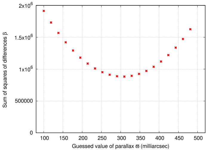
The "best-fit" value of the parallax is the value at which this graph shows a minimum value. It appears to be around 306 mas or so.
In order to find a more precise value, there are two common ways to continue the analysis:
Let's take the second option. After ten iterations of gradually re-centering the range, shrinking the limits, and making the grid spacing smaller and smaller, we end up with this graph:
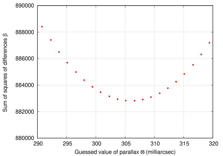
The "best" value for parallax appears to be ϖ = 306 mas, with a corresponding β value of about 0.88 million. If we adopt this value for parallax and generate predictions from our model, we find

Of course, we've been concentrating on just one (1) of the five (5) model parameters that we wish to determine. In addition to the parallax, we need to find the best values for proper motion in each direction, as well as the offset from our assumed initial position in each direction. The graph above shows very clearly that at least one of these other parameters does NOT have the value (zero) that we assumed earlier: the predicted Dec positions are systematically smaller than the measurements during the first half of the study period. That means that the value of L ought to be some positive number, perhaps 30 or 50 mas.
How can we fit all these other parameters? We can use the same sort of grid-based, try-them-all approach that we used for the parallax. However, we must watch out for a subtle factor in our implementation. An obvious way to proceed would look like this:
(iterate as many times as desired)
The danger with this approach -- replacing each guess with its new value as soon as we find it -- is that our numerical search might settle into some local minimum value of β, rather than finding the true global minimum. It might not happen, but if there is a significant correlation between two or more parameters, re-setting one might bias another in some direction away from the overall best fit.
So, a safer approach is to keep using a complete set of guesses in order to search for new parameter values, and then to update the values all at once. In other words, use an approach like this:
(iterate as many times as desired)
After 10 iterations of this safer algorithm, we end up with the following parameter values:
The model now runs through the middle of the measurements,

and the sum-of-squares-of-differences has shrunk down to a value of 0.18 million. This looks pretty good!
We've only discussed one of the two main methods to find the best-fitting parameters so far, but let's pause for a moment to consider a real-world complication: imperfect measurements. Take a look again at our measurements of the position of GX And.
Each measurement has errorbars in both the RA and Dec directions. The very last measurement at upper right, for example, has
    ΔRA   =  3185.5  +/-  88.3
    ΔDec  =   481.1  +/-  55.7
The change in RA for the star might have been 3185 mas ... or it might have been 3200 ... or 3230 ... or 3150. On the other hand, it's very unlikely that the true value was as large as 3400, or as small as 2800. When we compute the β statistic, we ought to account for this possible range in each direction.
To do so, we can change the sum from a simple "sum of squares of differences" to a WEIGHTED sum, like so:

With this modification, each of the RA and Dec terms in the sum will be -- roughly -- between 0 and 1 if the model is a good fit to the data, or considerably larger than 1 if the model is a poor fit. So, for example, if we compute β for a set of 10 measurements, a value of less than 20 suggests that the model does a good job of matching the measurements, while a value of 50 or 80 or more indicates that the model has some flaws.
It is slightly awkward to write equations with large expressions in fractional form, so let's define some weights based on the uncertainties in each measurement.

We can now write the equation for β in a somewhat more compact form:

We can use exactly the same grid-based method described earlier to find the parameters which minimize this weighted version of β. If we go through that same process, we find results that are roughly similar,

but do have a few differences.
| Quantity | Unweighted grid | Weighted grid |
| ϖ | 271 | 258 |
| μα | 2875 | 2893 |
| K | -36 | -30 |
| μδ | 405 | 411 |
| L | 80 | 74 |
| β | 180,000 | 57.4 |
First, note that while each parameter's value in the weighted column is similar to that in the unweighted solution, there are small differences. Why? Because some measurements count for more than others in the weighted solution, whereas all measurements have the same influence in the unweighted solution. For example, consider the four measurements with RA values between 1800 and 2000 mas: the two with larger Dec values have small errorbars, while the two with smaller Dec values have large errorbars. The unweighted solution will give all four equal weight, and so choose parameters which cause the model to run directly between the four measurements. The weighted solution, on the other hand, will choose parameters which lead to a model running further North, closer to the two measurements at larger Dec values.
Second, note the enormous difference in the value of β; instead of adding up squares of differences in milliarcseconds -- which were typically 50 or 100 each -- the weighted solution adds squares of differences in standard deviations -- which should each be of order 1. Our dataset includes measurements on 31 nights, each of which includes an RA value and a Dec value. So, IF
then we can expect that each term in the sum for β will contribute a number of order 1 for the RA factor, and another number of order 1 for the Dec factor. Thus, if we've chosen a good model, and estimated the instrumental uncertainties properly, we can expect to find a final value of β ≈ 31 × 2 ≈ 62. Lo and behold, our value of of 57 is right in this ballpark.
Some readers may have figured out that our weighted version of the quantity β is identical to the classical χ2 statistic. In this particular example, we have N = 62 measurements, m = 5 fitted parameters, and so ν = N - m = 57 degrees of freedom. The value χ2 = 57 means that our reduced chi-square value is χν2 = 1.0, which indicates that our model is a good match to the data, and that our uncertainties have been estimated correctly.
We've seen one way to find the parameter values which minimize the β statistic: iterate over many, many possible values of each and find the set which yield the smallest result. It's easy to understand and explain, not too hard to implement in code, but rather time-consuming to execute.
Let's now look at a completely different approach, which is considerably more complicated to derive, and no simple matter to implement, but which may run to completion more quickly. It is based on a fact that you may recall from an early calculus course.
At the minimum (and maximum) values of a function f(x), the first derivative is zero: df/dx = 0.
We are interested in finding the values of our five parameters which cause β = 0, so "all" we need to do is to find the values for which

It will turn out that this task will require us to do a bit of matrix arithmetic, but let's walk through the process to see how matrices come into it. For simplicity's sake, I will go through the derivation IGNORING UNCERTAINTIES, but then add them back at the end.
We begin with the definition of the sum-of-squares-of-residuals:
We'll treat of the five parameters in turn. Let's start with the parallax. The partial derivative of β with respect to ϖ is

The best fit will occur when this derivative is zero

which means that after dividing both sides by -2, we require

Re-arranging the terms a bit, we can write this as

Pause for a moment and examine the structure of this equation.
We will see exactly the same structure in each of the differential equations for the other parameters to be fit (though in a few, some of the terms on the left-hand side will be zero). The identical nature of the equations will allow us to combine them in matrix form. To make it easier to keep track of these items which will lead to the matrix formulation, I'll add a number on the far right side of each of these special equations.
But let's contine with the process. Next is the derivative with respect to the proper motion in RA.

Setting it to zero, and dividing by -2, yields

which we can re-arrange as

Note that in this case, the left-hand side contains terms for only three of the five parameters. We can force it into the standard form by adding terms for the two missing parameters, each multiplied by zero.

We can repeat these same steps for the proper motion in Dec.


Next, set the derivative with respect to the initial offset in the RA direction to zero.


Note that the "standard" form of this equation has a term for the parameter K in which the sum simply counts the number of measurements. If there are N measurements of the stellar position, that term could be written as K × N. However, we'll leave it in the summation form so that it looks similar to all the other terms.

Finally, set the derivative with respect to the initial offset in the Dec direction to zero.


Phew. That took a while, but all the work will pay off if we write the five numbered equations together, one right after the other.

Note that every one has exactly the same structure: five terms on the left, in each of which a single parameter to be fit appears to the first power. That means that we can express this set of mathematical equations in a matrix form, like so.

That's a pretty big and complicated equation. We can make it much more compact if we define three new variables: the big matrix A

the vector of parameters to be fit, x,

and the vector on the right-hand side, b.

With these definitions, the five conditions leading to the minimum value of the sum-of-squares-of-residuals becomes

That was a lot of work, but it pay off very quickly. Once we've computed all the terms in the matrix A and vector b, it takes just two steps to find the best-fit values for all five parameters.

Before we put this method into effect and solve for the best-fit values of the five parameters, let's go back to the beginning to add one last complication: accounting for the uncertainties in the measurements. Recall that we have defined weights for each measurement:
We can modify the equation for the β statistic to include these weights like so:
Taking the derivative of this expression with respect to each of the five parameters yields results very, very, similar to those we calculated above. The weights simply appear as additional multiplicative factors. For example, the derivative with respect to the parallax ϖ becomes

And thus

All terms referring to the RA measurements now include a factor of wRA2; and likewise, for terms referring to the Dec measurements, there is now a factor of wDec2.
This means that the matrix A becomes a bit more complicated,

as does the vector b

The method of solution remains the same: find the inverse of the matrix A, apply to the vector b, and *voila*, out pop the best-fit values of all five parameters.
| Quantity | Unweighted grid | Weighted grid | Weighted derivative |
| ϖ | 271 | 258 | 267 |
| μα | 2875 | 2893 | 2913 |
| K | -36 | -30 | -45 |
| μδ | 405 | 411 | 414 |
| L | 80 | 74 | 80 |
| β | 180,000 | 57.4 | 55.3 |
The model goes nicely through the middle of the measurements.

The results of the derivative-based method are very similar to those of the grid-based method; one has to look hard to see the small differences between them.

We've seen that there (at least) two methods to determine the values for the parameters in a model which will cause it "best" to match some given measurements. The results of the grid-based and derivative-based methods are very similar. This is all well and good, but leaves unanswered one very important question: Just how precise are the fitted parameter values? Are they perfect? Can we trust them to be within 1 percent of the true values? 10 percent?
There are a number of approaches one can take to estimate the uncertainty in some fitted parameter's value. I'll describe here just one, which I've chosen for its general nature. One can apply this idea to both the grid-based method and the derivative-based method; in fact, it ought to work with just about any technique at all. In my mind, this makes it a very powerful approach, and well worth the extra effort that it may require.
Look again at the recorded measurements for the position this star. Each set includes not only a value for RA and a value for Dec, but also an uncertainty in each of those values.
For example, the fourth measurement is
        motion in RA (mas)             motion in Dec (mas)
      ----------------------         -----------------------
         370  +/-  75                    162  +/-  89
That means that, even though we recorded an RA motion of 370 mas, the actual value might have been as small as 320, or 300; or it might have been as large as 420, or 430. Likewise, the Dec motion might have been anywhere between, roughly, 70 and 250 mas. Each of our measurements can be viewed as one possible random sample from within a range of possible measurements.
We can imagine a sort of "alternate universe" in which our instruments yielded a slightly different set of values from this range of possible measurements. We would have used the same telescope and same camera to observe the same target at the same location on the sky; the only difference would be the exact value of each RA and Dec coming out of the analysis. In one of these "alternate universes", the fourth measurement might have turned out to be
        motion in RA (mas)             motion in Dec (mas)
      ----------------------         -----------------------
         355  +/-  75                    211  +/-  89
Let's run with this idea, and create an entirely new set of measurements which are CONSISTENT with the actual measurements, by drawing random values from Gaussian distributions around the actual measurements. In the figure below, I show both the actual measurements (in red, with error bars), and the "alternate" measurements (in blue).

Of course, there's nothing special about this particular set of randomly chosen values. We could go through the same process again in another "alternate universe" and end up with a completely different set of "alternate" measurements which are, again, consistent with the actual ones.

For each "alternate" dataset, we can run one of our fitting programs to find the best-fit values of the five parameters. The results will be slightly different each time, of course. For example,
 Parameter               Actual       Alternate 1       Alternate 2
 ---------------------------------------------------------------------
  ϖ                       267              277              273
  μα                     2913             2927             2888
  K                       -45              -55              -28
  μδ                      414              403              380
  L                        80               78               96
 ---------------------------------------------------------------------
The range of fitted parameter values in the "alternate" datasets provides us with an estimate of the uncertainty in the fitted values of the parameters in the real dataset. More specifically, we can compute the standard deviation from the mean for each parameter, and use that as our uncertainty in the value of that parameter.
For example, generating 30 "alternate" datasets, and then applying the derivative-based method to each one in turn, yields parallax values which have a standard deviation of 18 mas away from their mean. We then conclude that the parallax value calculated from the derivative-based method should be ϖ = 267 ± 18. We can do the same for each of the five fitted parameters.
This very same approach can be applied to the grid-based method. Once again, we simply generate a number of "alternate" datasets, then run each one through our grid-based fitting program. Calculating the standard deviations from the means of the resulting parameter values yields estimates of the uncertainties in each parameter.
The table below shows the uncertainties computed in this way, using 30 "alternate" datasets for each method.
| Quantity | Weighted grid | Weighted derivative |
| ϖ | 258 ± 10 | 267 ± 18 |
| μα | 2893 ± 25 | 2913 ± 62 |
| K | -30 ± 10 | -45 ± 25 |
| μδ | 411 ± 33 | 414 ± 48 |
| L | 74 ± 14 | 80 ± 17 |
| β | 57.4 | 55.3 |
The uncertainties derived for the grid-based method are systematically smaller than those for the derivative-based method. Hmmmmm.
Note that, for all five parameters, the two different methods produce best-fit ranges which overlap each other. It's good to see that these two method are at least consistent with each other at the one-sigma level.
But are they CORRECT? Do these estimates and ranges contain the TRUE values of each of the parameters? In most experiments, it's not possible to answer this question, since one doesn't know the TRUE value of any quantity of interest. In this particular case, though, we are lucky. The European Space Agency's Gaia satellite has been scanning the sky since 2013, making many, many measurements of the position of most stars down to magnitude 19 or so. Each one of its measurements is much more precise than ours, and its observations cover a much longer timespan. In short, it has made such accurate and precise measurements of GX And (as well as of billions of other stars) that we can take its results as the truth.
The table below compares our results to those from Gaia.
| Quantity | Weighted grid | Weighted derivative | Gaia DR3 |
| ϖ | 258 ± 10 | 267 ± 18 | 280.70 ± 0.02 |
| μα | 2893 ± 25 | 2913 ± 62 | 2891.52 ± 0.02 |
| K | -30 ± 10 | -45 ± 25 | -- |
| μδ | 411 ± 33 | 414 ± 48 | 411.83 ± 0.01 |
| L | 74 ± 14 | 80 ± 17 | -- |
| β | 57.4 | 55.3 | -- |