 Copyright © Michael Richmond.
This work is licensed under a Creative Commons License.
Copyright © Michael Richmond.
This work is licensed under a Creative Commons License.
Yesterday, we started our trip up the distance ladder of astronomical distance measurements. Our method, parallax, is a very reliable one, but it doesn't reach very far ...
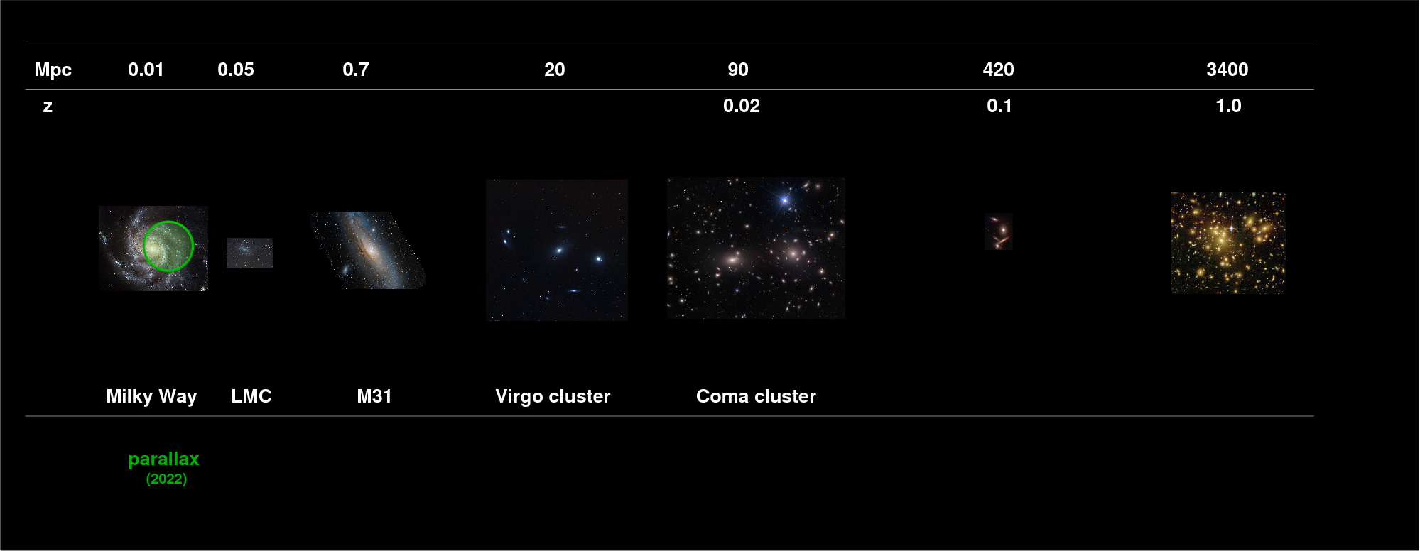
So, today, we'll take the second step up the distance ladder, using ordinary stars to measure distances RELATIVE to those already known from parallax.
If we want to measure distances to stars more distant than those for which parallax is reliable -- in other words, if we want to measure distances larger than a few hundred pc (as of 2017) -- then we have to give up a precious concept: that of absolute distance. Everyone agrees on the size of our Solar System and the length of the AU, and everyone accepts the simple trigonometry involved in the calculation of parallax, so the results of Hipparcos or Gaia are treated as "absolute": they rely on so few assumptions that, as long as the measurements are adequate, one can trust them completely.
But when we move up the next step of the distance ladder, we find ourselves considering relative distances. In every case, we will only determine the distance to object B in terms of the distance to some closer object A.
For example, we might measure the distance dA to a 100-Watt light bulb in our house, and note its brightness.
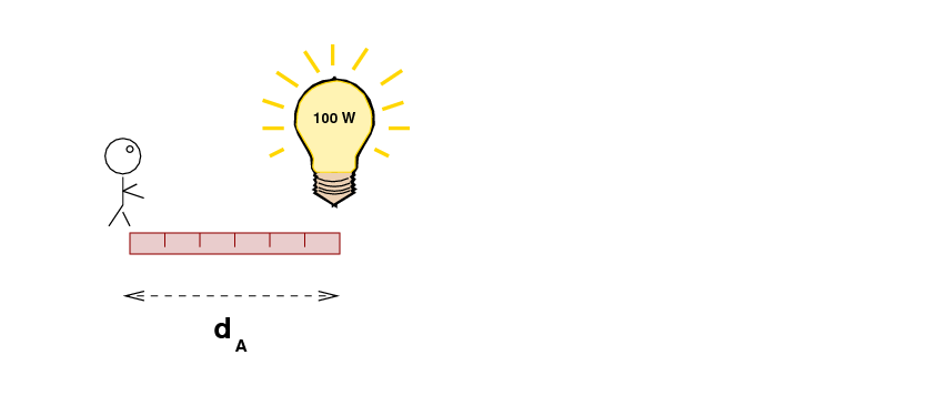
then carefully measure the brightness of a distant 100-Watt light bulb, at some unknown distance dB
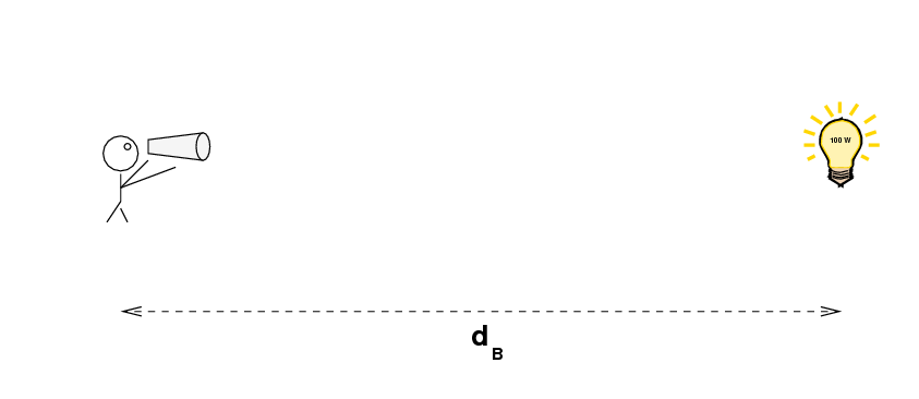
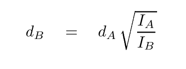
We can then use the inverse square law to compute the distance to the far-away light bulb:
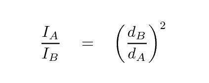
Of course, this means that any errors in the distance to A affect our estimate of the distance to B. That's the price of using relative distances, and the reason why the distance ladder becomes progressively less and less secure at larger distances.
One way to proceed is to pick one nearby star A, to which we have a precise distance from parallax, and one distant star B, to which we wish to determine the distance. In order to use a simple inverse-square law equation to compute the distance to B, we must pick stars which have the same luminosity. How can we do that?
Well, the best we can do is to pick two stars which are as similar in possible in
In most cases, though, when we try to find a nearby match for some distant star, we can only locate a star with approximately similar properties. That means that the two stars will probably not share exactly the same luminosity -- which means that our method to determine the relative distance will have some error.
Let's give it a try to see how well it works.
For our nearby star A, let's pick the Sun! We know the distance to the Sun perfectly (for all practical purposes), and we can measure all its properties very, very well.
For our distant objects B, I've chosen two stars which should be very good matches. They are "solar twins", taken from
The authors use very careful measurements of high signal-to-noise, high spectral resolution data to confirm 3 solar twins from one source, and identify 6 new solar twins from another. All the data is very high quality, so these matches are about as good as one can find. This is a "best case scenario" for measuring distances with a single pair of stars. Here are the two stars I've chosen from their set to compare to the Sun.
We'll start by making a table of the properties of these stars. I'll fill in the information for the Sun, using the apparent magnitude given by ( Mamajek's Star Notes); half the class will find the data for HD 78660, and the other half for HD 183658. First, we need to fill in the apparent V magnitude column. I recommend that you look in the Hipparcos catalog to find the Vmag (magnitude in Johnson V-band) for each star.
       star              apparent V magnitude         distance (pc)
 -----------------------------------------------------------------------

       Sun                    -26.71 +/- 0.02          4.84813 x 10⁻⁶

     HD 78660

     HD 183658

 -----------------------------------------------------------------------
Okay, once we've filled in the V magnitude column, it's time for you to figure out the distance to each of the solar twins, using the inverse square law.
Not sure how to find distance? Look here
Okay? Finished? You can see my values for the completed table if you want to compare your results to mine.
How well did this method work? We can find out by comparing these results to the distances derived by a better method: trigonometric parallax. It turns out that both of these stars are close enough, and bright enough, to have good measurements in the Hipparcos catalog.
So, please use the Hipparcos catalog to look up the parallax for each solar twin, and then compute its distance using that value.
                                               distance (pc) based on
       star             parallax (mas)       parallax         magnitudes
 -----------------------------------------------------------------------

     HD 78660

     HD 183658

 -----------------------------------------------------------------------
Finished?
When you are ready, you can see how your calculations compare to mine.
So we find that using the relative brightnesses of two stars, which we ASSUME to be identical, to compute their relative distances, sometimes yields the same answer as the (better, in general) trigonometric parallax technique ... but not always.
The trouble is that it's very difficult to find two stars which are perfect matches. And even if you can find an exact match, making a small random error in your measurement can ruin the result.
Using just one nearby star to determine the distance to one distant star is not easy, as we have seen. A better idea is to pick a BUNCH of local stars, and a BUNCH of distant stars, and compare the properties of these two groups to determine the relative distance between them. If we pick the groups carefully, we can address some of the problems that we encountered when trying to match single stars. Remember these?
All we need to do is to make one assumption:
     Assume: All the stars in a cluster are born at the same time
             from a cloud of gas which has uniform chemical composition.
With this proviso, the members of an open cluster or globular cluster provide us with an excellent set of subjects, one which reveals quite a bit about its age and metallicity.
When the stars are first born, they all lie on the main sequence of a Hertsprung-Russell (HR) diagram. Massive stars are hot and luminous, low-mass stars are cool and feeble. (Click on the figure below to activate it)
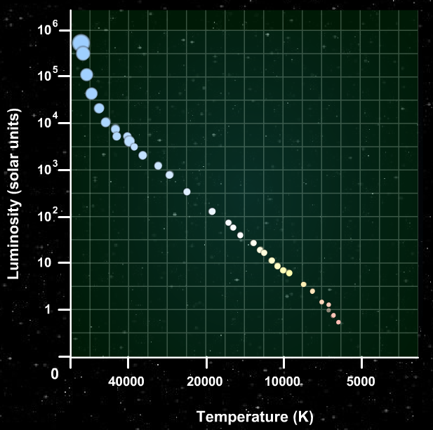
After 5 million years, the most massive stars run out of hydrogen in their cores and leave the main sequence, moving toward the red giant area of the HR diagram.
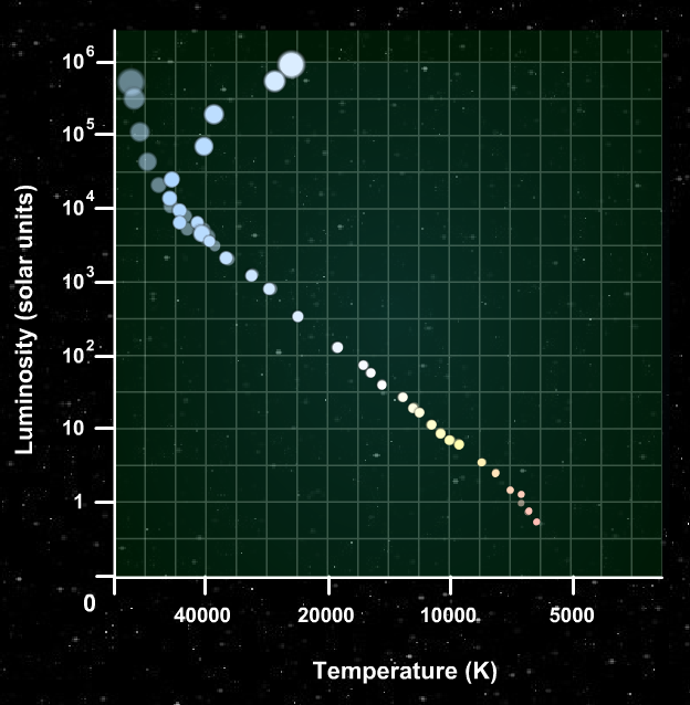
After 80 million years, the most massive stars are long since dead. Now less massive stars start to evolve off the main sequence ...
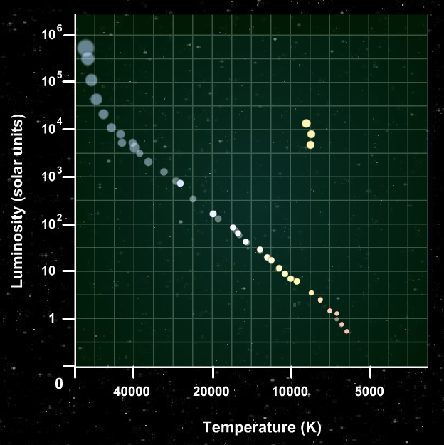
And after billions of years, only the low-mass members of the cluster remain on the main sequence.
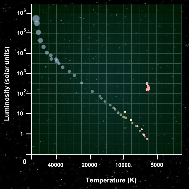
So we can estimate the age of a cluster of stars by looking at the location of the main-sequence turnoff on its HR diagram.
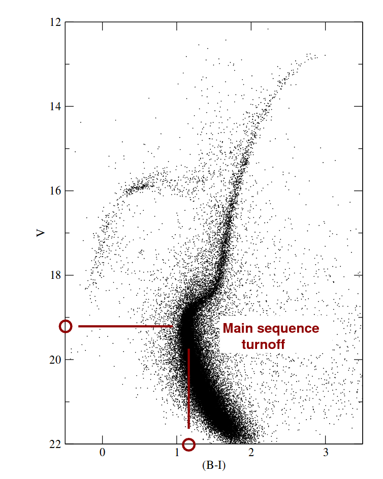
Image taken from Fig 3 of
Feuillet, Paust and Chaboyer, PASP 126, 733 (2014)
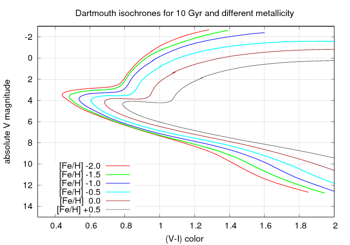
The change in shape of the HR diagram with age is pretty straightforward, but also relatively small after a few billion years. For globular clusters, for example, which typically have ages greater than 8 Gyr, look at the change with time; the figure below is based on isochrones (models of stars created with a particular age and metallicity) provided by the the Dartmouth stellar evolution group.
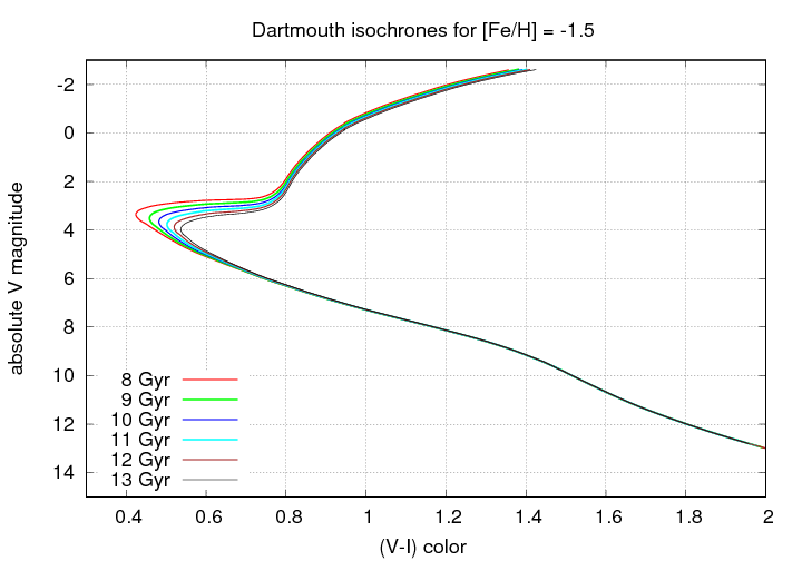
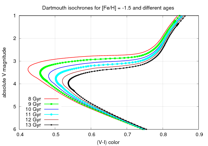
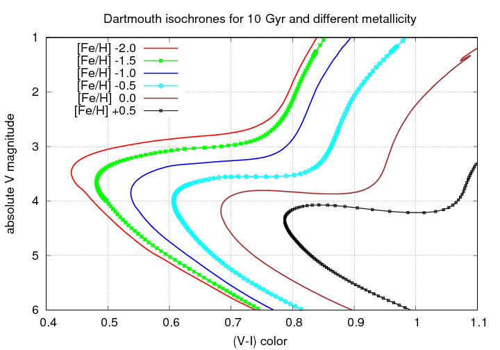
Let's zoom in to see more closely the region of the main sequence turnoff point:
But age isn't the only variable which can affect the luminosity of the stars in a cluster: the metallicity of the gas making up the stars can also have an important effect. A good illustration of this point is given by Ross et al., AJ 147, 4 (2014). In their Figure 8, they show color-magnitude diagrams for 5 globular clusters with a range of metallicities, ranging from the very metal-poor M92, [Fe/H] = -2.3, on the left, to the metal-rich NGC 6791, [Fe/H] = +0.4, on the right.

Figure 8 taken from
Ross et al., AJ 147, 4 (2014).
  Q:  What features in these HR diagrams
      change with metallicity?
I can see at least three pretty obvious features:
Note that the first feature, the color of the turnoff point, can be affected by reddening; so one has to be very careful to measure the extinction to the cluster properly. But the other two indicators are relatively reddening-independent, which makes them easier to apply in many cases.
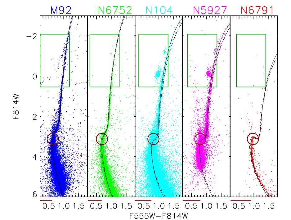
Figure 8 taken from
Ross et al., AJ 147, 4 (2014).
The authors of the paper compare the main-sequence turnoff point to a number of isochrones with different metallicity. What short of changes occur in the HR diagram of a cluster as a result of metallicity? Let's take a look:
That's a much larger change than we saw with ages. Again, let's zoom in to look at the main-sequence turnoff point:
In the figure below, which uses a color based on the HST F390M and F555W filters, which is similar to (B-V), you can see the location (in color) and shape of the main-sequence turnoff change very clearly with metallicity. The solid black lines in the diagram are isochrones from the Dartmouth stellar isochrones; the model for M92, for example, has an age of 13.5 Gyr and a metallicity of [Fe/H] = -2.3.
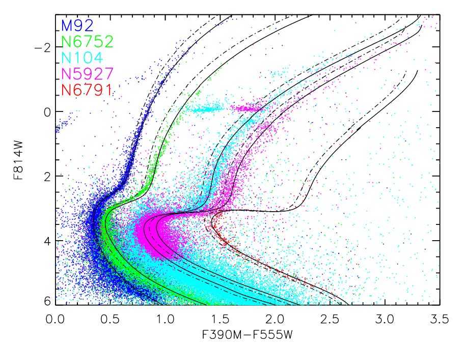
Figure 11 taken from
Ross et al., AJ 147, 4 (2014).
So, if we measure the properties of a large number of stars in a single cluster, then we can use the HR diagram to figure out the age and metallicity of all the stars in the cluster. Then, if we find another cluster with similar properties, we can safely use the offset between some feature in the HR diagram to measure the relative distance between the clusters.
If you study clusters in detail, you'll want some way to convert the observed properties (magnitudes and colors) into physical properties of the stars (ages, masses, metallicities). Computing stellar models is a complicated business, so it makes sense to use the results of experts.
The Darthmouth Stellar Evolution Database provides you with a web-based interface that allows you to generate models according to your own preferences, then download the resulting isochrones. Let's give it a try to see how this works.
First, go to the The Darthmouth Stellar Evolution Webtools webpage and click on Isochrones and Luminosity Functions (2012 Update). You should see a page like the one below.
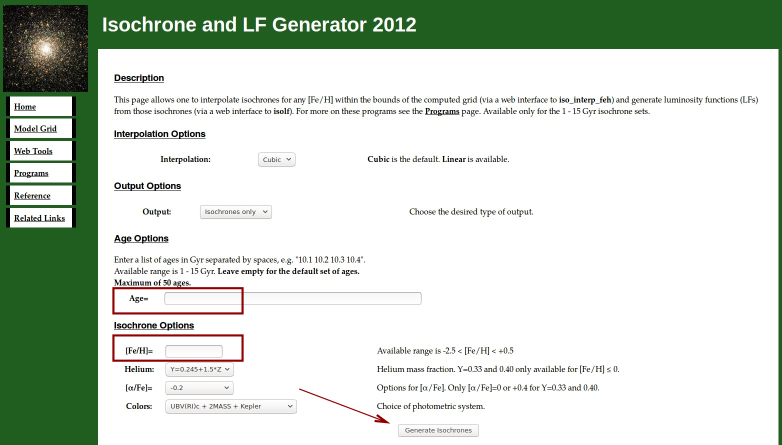
You should receive shortly a small ASCII text file. Download it to your computer, and examine it with any text editor. You'll see something like this:
#NUMBER OF AGES= 1 MAGS=10
#----------------------------------------------------
#MIX-LEN  Y      Z          Zeff        [Fe/H] [a/Fe]
# 1.9380  0.2457 4.2021E-04 5.4961E-04  -1.50  -0.20
#----------------------------------------------------
#**PHOTOMETRIC SYSTEM**: Bessell UBV(RI)c + 2MASS JHKs + Kepler (Vega)
#----------------------------------------------------
#AGE= 1.000 EEPS=265
#EEP   M/Mo    LogTeff  LogG   LogL/Lo U       B       V       R       I       J       H       Ks      Kp      D51
   3  0.120104  3.5404  5.2921 -2.6595 16.2798 14.5182 12.7685 11.7602 10.8176  9.6603  9.0819  8.9366 11.9153 13.5298
   4  0.131716  3.5478  5.2487 -2.5461 15.7054 14.0989 12.4097 11.4270 10.5304  9.3988  8.8112  8.6567 11.5941 13.1330
   5  0.149993  3.5576  5.1986 -2.4008 15.0161 13.5661 11.9549 11.0037 10.1588  9.0619  8.4681  8.3041 11.1822 12.6305
   6  0.186126  3.5719  5.1440 -2.1953 14.1011 12.8213 11.3156 10.4138  9.6283  8.5844  7.9904  7.8160 10.6010 11.9290
   7  0.240633  3.5859  5.0886 -1.9725 13.1982 12.0522 10.6435  9.7932  9.0539  8.0618  7.4730  7.2934  9.9825 11.1981
   8  0.289720  3.5946  5.0510 -1.8190 12.6106 11.5410 10.1895  9.3731  8.6593  7.6992  7.1155  6.9358  9.5619 10.7075
Columns 8 and 10 contain the "V" and "I" magnitudes for the model stars; each line shows the properties of stars with a different mass.
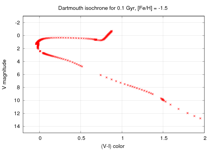
  Q:  Can you make an HR diagram using this datafile?
      Use "V" magnitude on the vertical axis and the
      difference "(V-I)" on the horizontal axis.
An example I made is shown below.
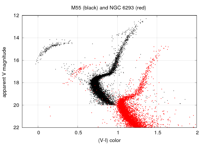
Let's put all this theory into practice. We'll start with one globular cluster, M55, which has a known distance: 5.4 kpc. Suppose we want to measure the distance to the cluster NGC 6293.
Yes, yes, astronomers have measured the distance to this cluster already. Just play along, okay?
Our first job is to create HR diagrams for each of these clusters. Fortunately, both have data in the wonderful Vizier system. You can find the data with a simple search by the cluster name. I've already done that:
In fact, I grabbed the data and edited it a bit, throwing away most of it (and good stuff, too!), leaving just the bits you need to make an HR diagram. Each datafile has a two-column format, with the V-band magnitude in column 1 and the I-band magnitude in column 2, like this:
#RESOURCE=yCat_51322171
#Name: J/AJ/132/2171
#Title: VI photometry of NGC 6293 and NGC 6541 (Lee+, 2006)
#Table J_AJ_132_2171_table3a:
#Name: J/AJ/132/2171/table3a
#Title: Color-magnitude diagram data for NGC 6293
#
#  V      I
17.648 16.194
18.108 16.689
19.499 18.197
19.493 18.397
19.231 17.999
Your job is to do the following:
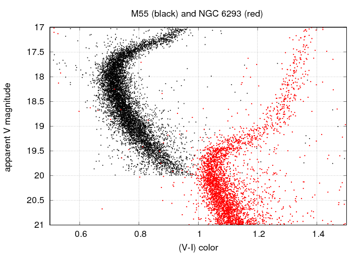
If you are having trouble, you might want to peek at this graph, or maybe even zoom in on the main-sequence turnoff.
Q: What distance did you determine for NGC 6293?
I have read that the actual distance is about 8.4 kpc. I suspect that your value is quite a bit larger.
  Q:  Can you think of any effect that we might have ignored
      in our calculation?
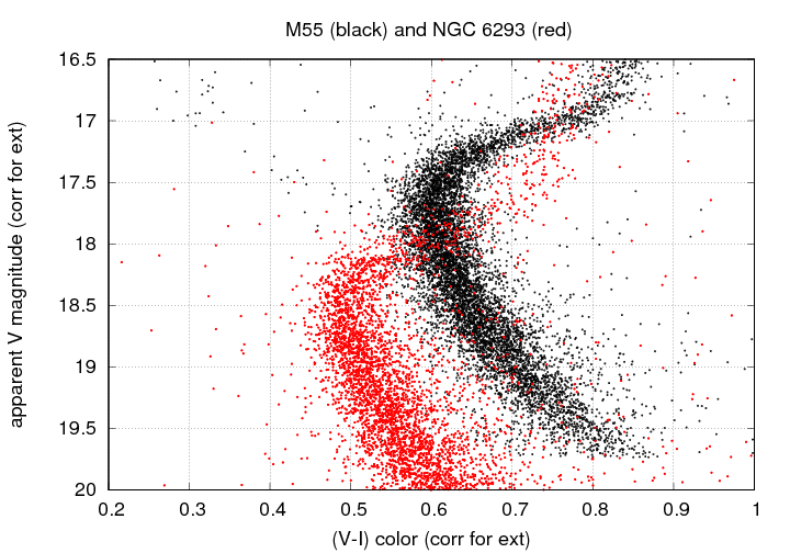
Yes! That's right. Extinction! The values in these catalogs are observed magnitudes, not corrected for extinction due to dust and gas along the line of sight.
I looked up the estimate of that extinction for each of these clusters, finding values of
   cluster      E(B-V)      A(V)     A(I)      A(V)-A(I)
  -------------------------------------------------------
     M55         0.08       0.265    0.155      0.110

   NCC 6293      0.40       1.326    0.776      0.550
  -------------------------------------------------------
In order to correct for this extinction, you must subtract the value in the A(V) column from the V-band magnitudes on the y-axis, and subtract the value in the A(V)-A(I) column from the (V-I) colors on the x-axis.
  Q:  Can you make a new version of your HR diagram,
      incorporating these corrections?

      What is the difference in V-band magnitude
      for the main-sequence turnoff now?
If you don't know how to make the changes, or don't have time, you could just look at my corrected version.
  Q:  Using this new difference in magnitudes,
      and the 5.4 kpc distance to M55, what is the
      distance to NGC 6293?


      How does it compare to the literature
      value of 8.4 kpc?
In order to tie the RELATIVE distances of clusters to an ABSOLUTE scale, we need to know the real distances to some nearby star clusters via parallax. Back in the "old days", this was not so easy. Astronomers spent many years working on a few nearby clusters, trying very hard to avoid systematic errors and cross-check their results.
Two of the most commonly used nearby clusters are the Hyades and the Pleiades, both relatively young open clusters, both visible to the naked eye in the winter sky. We can see our estimates of the distance to the Hyades have not changed (much) over the last few decades:
 year    method           distance              reference
-----------------------------------------------------------------

 1967    parallax,
         emission lines,
         convergence,      48.3                Hodge and Wallerstein, PASP 78, 411 (1966)

 1967    revised           44.3                Wallerstein and Hodge, ApJ 150, 951 (1967)


 1997    FGS parallax      46.1                van Altena et al., ApJ 486, L123 (1997)

 1997    binary star       47.4  +/- 2.3       Torres et al., ApJ 479, 28 (1997)

 1998    Hip parallax      46.34 +/- 0.27      Perryman et al., A&A 331, 81 (1998)

 2017    Gaia parallax     46.75 +/- 0.46      Gaia Collab, A&A 601, A19 (2017)


-----------------------------------------------------------------
The most recent paper in that table , published just a few months ago, presents analysis of the distances to 19 open clusters, including the Hyades and Pleiades. We can now make accurate HR diagrams for a number of clusters, allowing us to use them for relative distance measurements, AND allowing us to check our models of stellar evolution.
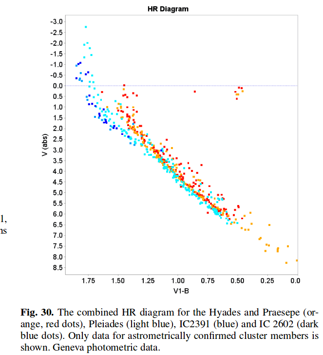
Figure 30 from
Gaia Collab, A&A 601, 19 (2017)
Copyright © Michael Richmond.
This work is licensed under a Creative Commons License.