 Copyright © Michael Richmond.
This work is licensed under a Creative Commons License.
Copyright © Michael Richmond.
This work is licensed under a Creative Commons License.
We see transits because a planet passes in front of its host star as it revolves in its orbit. Alas, all stellar systems are so far away that we can't resolve the star and "see" the little black spot of the planet directly. In other words, we CANNOT see something like this:
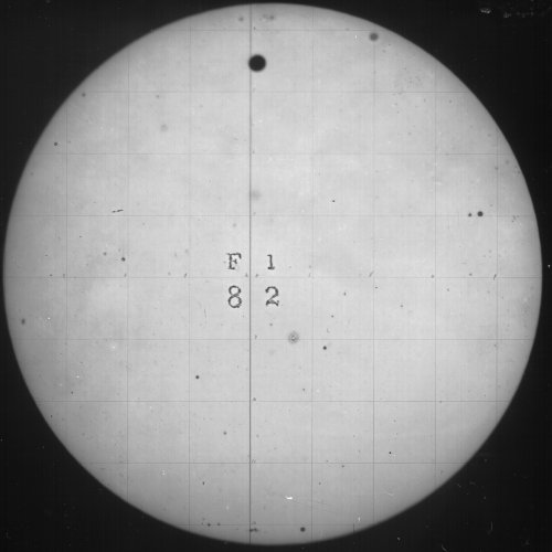
A picture of the transit of 1882, from
the US Naval Observatory's Rare Books collection.
All we know is that the planet
It seems impossible for us to determine which way the planet was moving.
Of course, we know which way the planet ought to be orbiting its host star: in the same direction that the star itself is rotating. After all, if the star and the planet formed out of the same primordial disk of material, then they ought to have angular momentum pointing in the same direction.
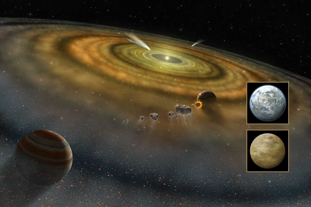
Image credit: Lynette Cook
  Q:  Is there any way to figure out if the planet is orbiting
          in the expected direction?
Yes, of course. Why else would I ask the question?
The key is to take spectra of the star several times during a transit and look for a subtle effect.
Way back in the early 1920s, a pair of graduate students at the University of Michigan were studying binary stars. They used the Ann Arbor 37.5-inch reflecting telescope to take photographic spectra of bright stars.
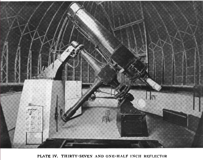
Image taken from
Publications of the Astronomical Observatory of the
University of Michigan, Vol 1 (1912) ,
thanks to Google books.
Richard Alfred Rossiter observed the binary star beta Lyrae (V = 3.42) for his dissertation. He combined a series of his own measurements with a series taken earlier at Michigan, as well as a set taken back in 1907 at the Allegheny Observatory in Pittsburgh. His paper describing the system
points out a small deviation of the measured radial velocities from the expected pattern:
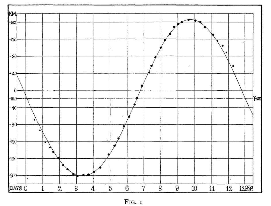
Figure 1 taken from
Rossiter, ApJ 60, 15 (1924)
The deviations are largest right around the primary eclipse, near day 0 or day 13 in the figure above. Rossiter plotted the residuals from the smooth curve as a function of phase.
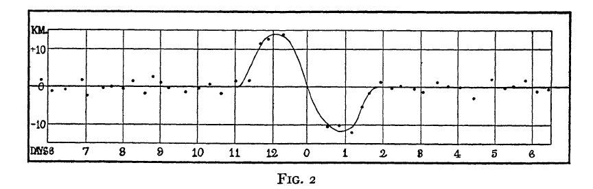
Figure 2 taken from
Rossiter, ApJ 60, 15 (1924)
Note the pattern: a redshift before the eclipse, followed by a blueshift after the eclipse. Rossiter had an explanation for this pattern, which we'll read in just a moment.
This work would earn Rossiter his Ph.D. in 1924.
Meanwhile, a younger student at Michigan, Dean Benjamin McLaughlin, was just 23 years old; he might have just been starting his graduate work at this time. He used the 37.5-inch telescope to observe a different bright binary star: Algol (V = 2.12).
He published his results in the very same issue of ApJ as Rossiter; in fact, his article was on the very next page.
McLaughlin combined his own spectra with those from earlier observers at Michigan and a few from the earlier literature. He and Rossiter were clearly working together and talking about this small pattern of discrepant radial velocities, as he writes
By far the most numerous group is that of the present season, which includes 79 plates. Of these, 39 were used for the determination of the orbital elements of the binary system; the remaining 40 were taken for the express purpose of investigating this effect of the star's rotation discovered by Dr. Rossiter in Beta Lyrae.
The exposure times for the each spectrum were likely around one hour, so this effort was ... considerable.
McLaughlin found that the radial velocities of Algol showed a pattern like that of beta Lyr. Around the time of eclipse, there was a deviation from the smooth sine curve of radial velocities; the residuals looked like this:
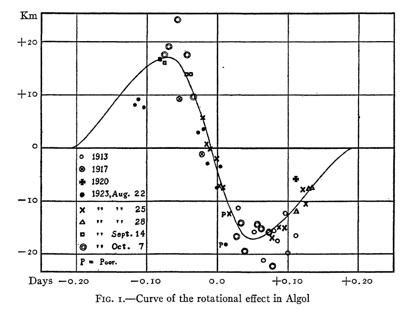
Figure 1 taken from
McLaughlin, ApJ 60, 22 (1924)
  Q:  What was causing this pattern of small changes
         in radial velocity during an eclipse?
Rossiter found an explanation for this effect. Let's read it.
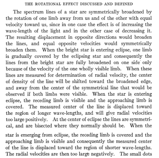
The key is recognize that we USUALLY see light from both limbs of a rotating star: one side coming toward us, the other moving away. The light from the approaching side is slightly blueshifted, and that from the approaching side is slightly redshifted. Hence, each spectral feature is broadened.
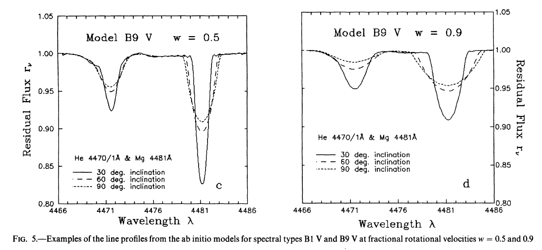
Figure 5 taken from
Collins and Truax, ApJ 439, 860 (1995)
But, during an eclipse, as one star passes in front of the other, it will block the light from one limb, removing the photons which have been shifted in one direction. That will leave the overall mix of photons unbalanced, resulting in a shift in the apparent wavelength as long as one limb is blocked.
This is one of those cases in which a picture (or, perhaps, several pictures) is worth a thousand words.
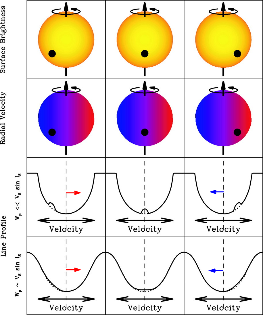
Figure 1 taken from
Gaudi and Winn, ApJ 655, 550 (2007)
Well, there's nothing really mysterious about this effect, but it's a subtle one. It's especially subtle when the eclipsing body is a tiny little planet instead of a companion star: instead of covering HALF the disk of the primary star, the planet might cover ONE-THOUSANDTH of the disk. Any variation in the observed radial velocity of the primary star will be hard to find.
So, why bother?
The answer lies in ... well, let's find out the fun way.
It's the Rossiter-McLaughlin Effect Game Grid!
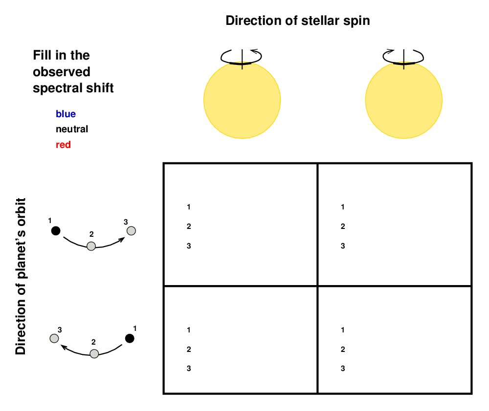
Yes, that's right: as one measures the shift in radial velocity over the course of a single transit, one will see one of two possible patterns:
So, if we can measure the radial velocity of a star with VERY HIGH PRECISION over the course of a transit, we can figure out the direction of the transiting planet's orbit.
Let's look at one example:
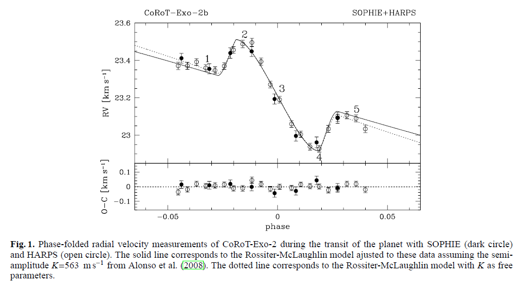
Figure 1 taken from Bouchy et al., A&A 482, 25 (2008)
  Q:   What is the systemic radial velocity of the host star?


  Q:   How large are the Rossiter-McLaughlin variations?
          Is this an easy measurement?


  Q:   Is the planet in this system in a prograde or retrograde orbit?
In fact, the RM effect can reveal not only the direction of the planet's orbit, but also its inclination λ relative to the spin axis of the star.
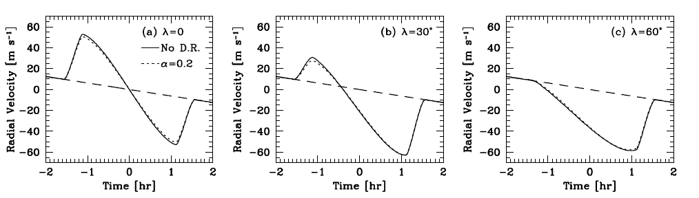
A portion of Figure 4 taken from
Gaudi and Winn, ApJ 655, 550 (2007)
Thanks to the exoplanets.org website , one can quickly examine the properties of known exoplanets, including the values of
λ = (star's spin axis angle) - (planet's orbital axis angle)
Nota bene: it is necessary for the user explicitly to add λ to the list of quantities shown in tables and in graphs, as it is not one of the default quantities. That's not surprising, as only
Let's look at the spin-orbit misalignment in these 69 systems:
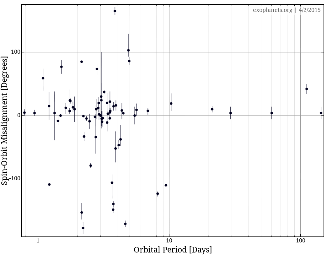
Q: Do you see any surprises here?
I surely do!
Almost half (30 out of 69) systems have a misalignment of at least 20 degrees -- even systems with planets orbiting at very small separations from their stars.
If these systems formed as planets accreted from a disk around the star, and (especially?) if some of these "hot Jupiters" migrated inward through the last remains of that disk ... then how did they end up in orbits SO INCLINED to that disk?
One possibility that is raised in some papers which measure the misalignment is the Kozai mechanism.
There are lots of other possible mechanisms, such as planet-planet scattering, but let's leave those for another time.
Back in 1962, Kozai studied a particular subset of the three-body problem:
Kozai found that under certain circumstances, the orbit of the asteroid can undergo cycles in which the values of its orbital eccentricity e and inclination i vary, but the quantity
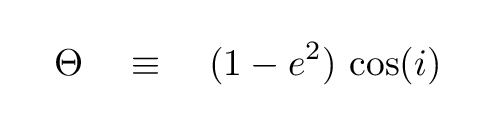
remains a constant.
As Kozai himself explains, 50 years after his paper , he was considering only the effect on the orbit of asteroids in our Solar System. Moreover, he realized that the timescales for these changes would be very long:
Since they are secular perturbations with a period of a few thousand years, nobody could detect them from observations of asteroids.
But, over the years, astronomers studying other systems -- multiple stars, and even collisions of galaxies in cosmological simulations -- realized that the same mechanism could come into play in the systems they studied.
If a 3-body system consists of two stars and a planet (so that here, the "tiny mass" asteroid of Kozai's original paper becomes the transiting planet),
then the period over which the planet's inclination will vary is given by the "Kozai time":
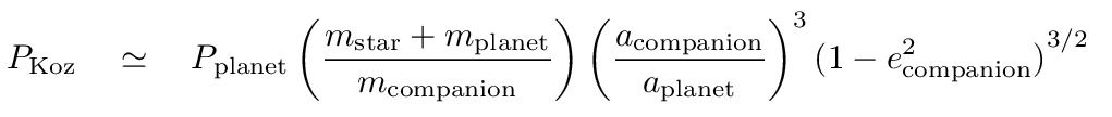
  Consider a "hot Jupiter" circling a Sun-like star with a period of 5 days,
      and a second Sun-like star, orbiting the first at a
      distance of 100 AU (or 1000 AU), with negligible eccentricity.


    Q:  What would the period of the "companion" be?


    Q:  What would the "Kozai time" be for this system?
Copyright © Michael Richmond.
This work is licensed under a Creative Commons License.