 Copyright © Michael Richmond.
This work is licensed under a Creative Commons License.
Copyright © Michael Richmond.
This work is licensed under a Creative Commons License.
In 2005, radial velocity measurements by Bonfils et al., A&A 443, L15 (2005) indicated that the nearby M dwarf Gliese 581 was accompanied by a Neptune-mass planet, Gliese 581 b. The evidence was solid.
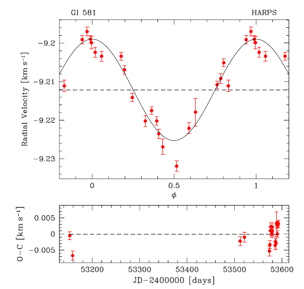
Figure 2 taken from
Bonfils et al., A&A 443, L15 (2005)
Q: What is the amplitude of the radial velocity variations?
Two years later, Udry et al., A&A 469, L43 (2007) showed that further observations of the system indicated the presence of two more planets. This brought the total to 3:
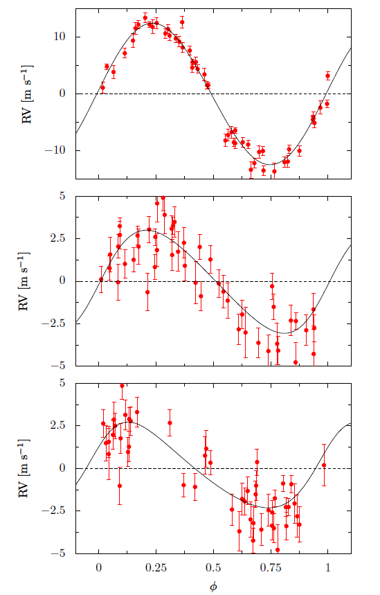
Figure 3 taken from
Udry et al. (2007)
Q: What is the amplitude of the radial velocity variations of planet 'd' ?
In 2009, things got really exciting when Mayor et al. A&A 507, 487 (2009) announced that, not only had they found evidence for a fourth planet (e), but a revised analysis showed that the third planet (d) was actually inside the habitable zone.
According to this paper, the tally was now
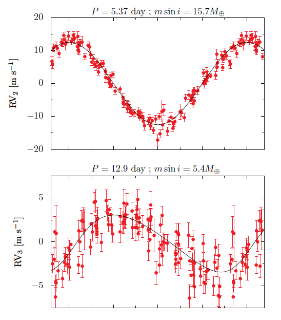
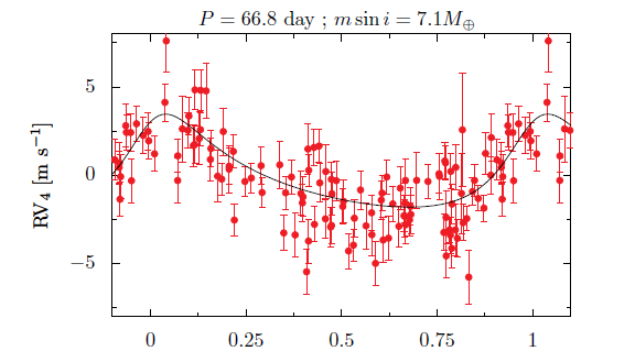
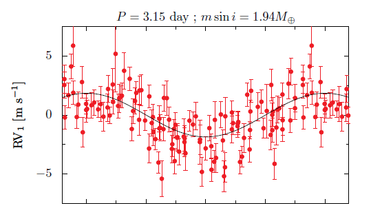
Figure 2 taken from
Mayor et al. A&A 507, 487 (2009)
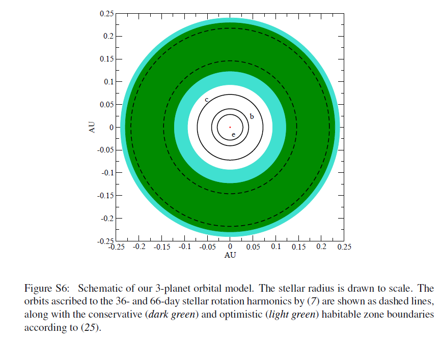
Figure S6 taken from
Robertson et al., Science 345, 440 (2014)
Now, for several years, things were a bit unsettled. Some scientists claimed that some of these planets might not be real detections; others claimed to find two MORE planets, 'f' and 'g'. Eventually, Robertson et al., Science 345, 440 (2014) put forth the claim that some of the variations in radial velocity of Gliese 581 might not be due to planets, but due to activity in the star's atmosphere.
After all, this M star has quite an active chromosphere, as the emission line in H-alpha shows.
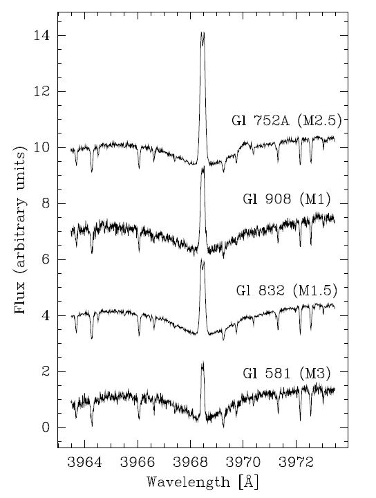
Figure 1 taken from
Bonfils et al., A&A 443, L15 (2005)
Spectral measurements of Gliese 581 suggest that the star rotates with a period of 130 +/- 2 days. Robertson et al. argued that the signal for planet 'd' (period = 66 days = half of stellar rotation period) was correlated so strongly with stellar activity (as indicated by the strenth of H-alpha emission) that there was no planet 'd'. They made a similar argument for the non-existence of planet 'g' (period = 33 - 36 days = one-quarter of stellar rotation period ).

Figure 1 taken from
Robertson et al., Science 345, 440 (2014)
Just a few days ago, Anglada-Escude and Tuomi, arXiv 1503.01976 pointed out that one facet of the analysis used by Robertson et al. (and LOTS of other astronomers) was done improperly; or, perhaps, less than optimally. They write:
Detecting a planet candidate consists of quanti- fying the improvement of a merit statistic when one signal is added to the model. Approximate methods are often used to speed up the analyses, such as computing periodograms on residual data. Even when models are linear, correlations exist between parameters. Similarly, statistics based on residual analyses are biased quantities and cannot be used for model comparison.A golden rule in data-analysis is that the data should not be corrected, but it is our model which needs improvement.
The point here is that it's dangerous to to search for periodic signals in a noisy dataset in the following manner:
Round 2:
Round 3:
etc.
Anglada-Escude and Tuomi warn that operating on a series of successive residuals is poor practice, because each of the fitting steps in this sequence will actually be influenced by both real effects (planets) and noise as well.
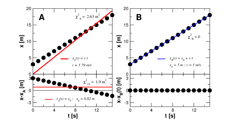
They provide a simple example: suppose that your job is to fit a model to some measurements, where your models look like this.
   simplest model:    y  =  a*x


   next model:        y  =  a*x  +  b
The question is -- does the data justify only the simplest model, or does it justify a more complex one?
They illustrate their argument with this figure. On the left is the result of the sequence
On the right is the result of the procedure
The authors go on to write about the "false-alarm probabilities (FAP)" discussed so frequently in the analysis of radial velocity variations.
derived false alarm probabilities would be representative only if a model with one-sinusoid and one offset is a sufficient description of the data, measurements are uncorrelated, noise is normally distributed, and uncertainties are fully characterized.Every single of these hypothesis breaks down when dealing with Doppler residuals: the number of signals in not known a priori, fits to data correlate residuals, and formal uncertainties are never realistic.
Copyright © Michael Richmond.
This work is licensed under a Creative Commons License.