 Copyright © Michael Richmond.
This work is licensed under a Creative Commons License.
Copyright © Michael Richmond.
This work is licensed under a Creative Commons License.
This week, we will take a "Big Picture" look at our knowledge of extrasolar planets:
A very good place to start is the overview provided by NASA at the Exoplanet and Candidate Statistics page:
Please take out an Internet browsing device, and follow along as we take a little trip. Pay careful attention: you'll have to answer some questions as we go.
If you set your browser to the Exoplanet and Candidate Statistics page and click on the item All Exoplanets at the bottom of the table, you should be taken to an interactive table that looks something like this:
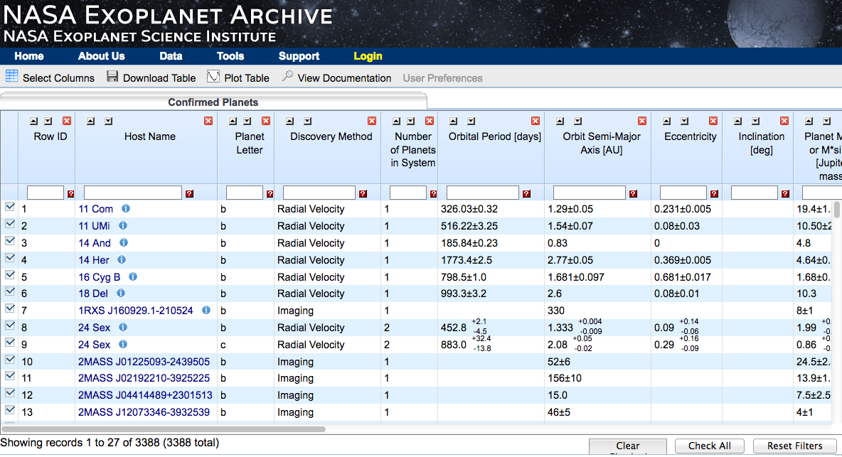
This table is interactive -- you can modify its contents by typing and clicking on various items. For example, we can select only the exoplanets which satisfy a certain numerical criterion by typing text into the boxes near the top of each column.
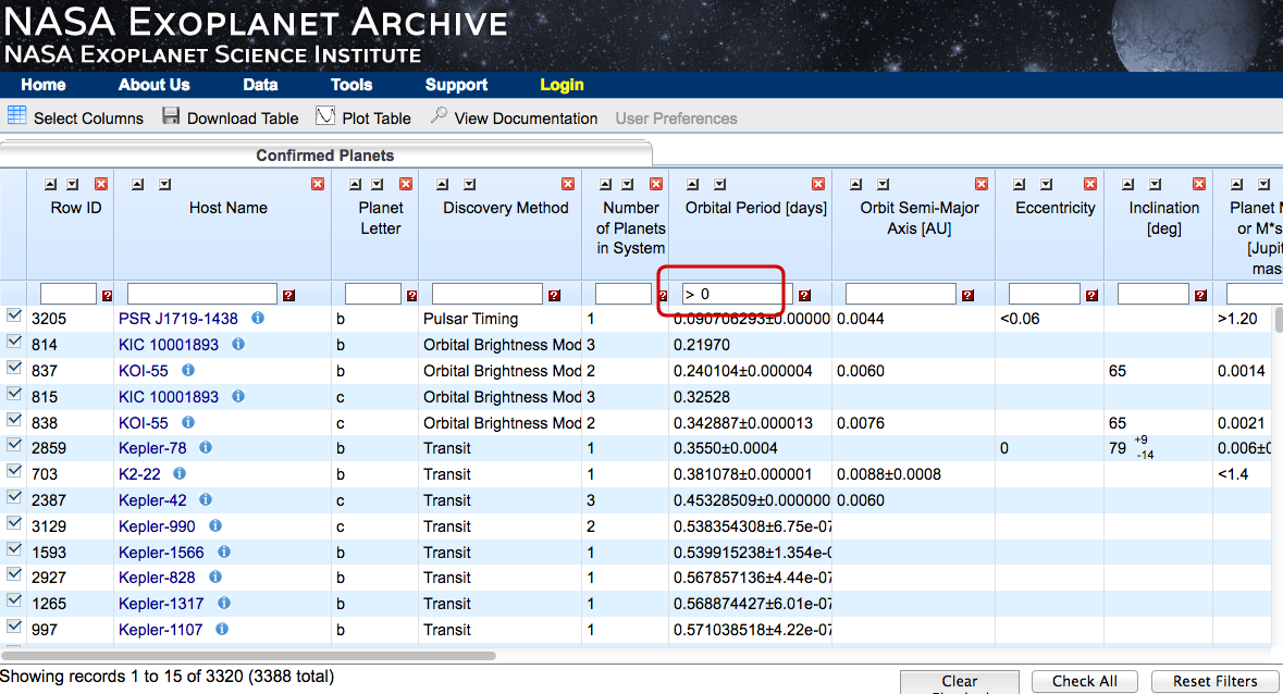
For example, I can choose only those exoplanets with measured periods by typing "> 0" into the box for "Orbital Period", like so:
Please use this method to answer the following questions:
   Q 1:   a) How many planets have a measured period?

          b) How many planets have a measured mass?

          c) How many planets have a measured radius?

          d) How many planets have a measured orbital radius?
Hmmmmm. It seems that some properties of planets are EASY to measure, but others are DIFFICULT. We will discuss some of the reasons for this over the next seven weeks -- but can you guess some of the reasons for these particular properties?
The first thing we see when we visit the page is that of the 3587 (as of Jan 23, 2018) confirmed exoplanets, the very great majority were found by the transit technique:
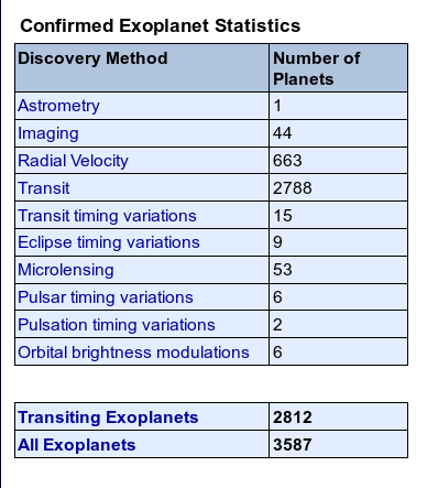
   Q 2:   Why has the transit method produced such a large fraction -- 78% --
             of the total?
Of the remainder, the bulk were discovered using radial velocity measurements: 18.4%, to be precise.
That leaves just a tiny amount, about 3.3%, for all the other techniques combined. That is one reason that we will spend more time on the transit and radial velocity techniques than on the others.
Okay, let's focus for a moment on the exoplanets found via the radial velocity method. Go to the the Exoplanet and Candidate Statistics page and click on the item Radial Velocity in the table.
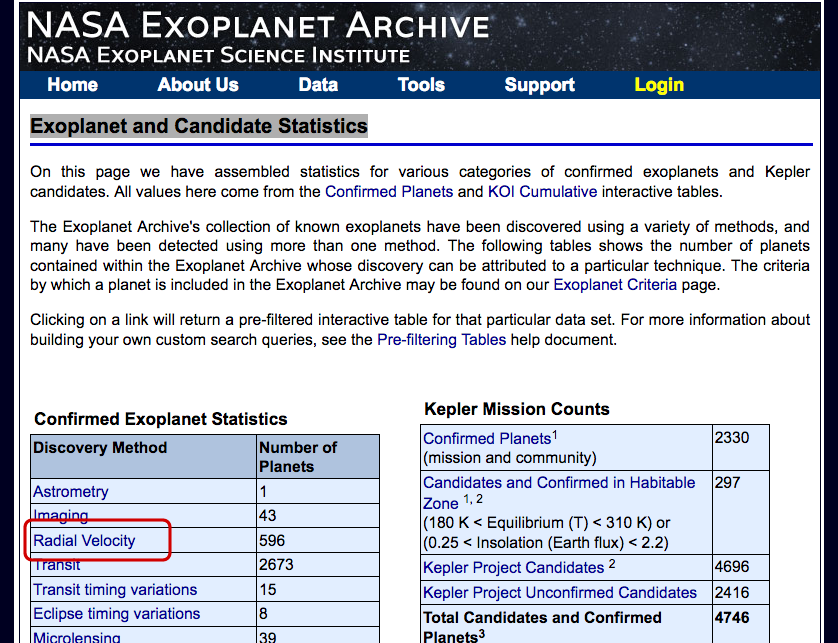
This will create an interactive table containing only exoplanets which were discovered by the radial velocity method.
Let's look at two particular entries in this table:
   Q 3:   Look at the periods of these two exoplanets.  Which one
          has been measured more precisely?


   Q 4:   Explain why one of them has a much less precise period.
So far, we can see that this table provides lots of useful information -- just like any ordinary table. But NASA has done a very nice job in making the table an interface into a very rich database. If you place your cursor over the "i" icon next to an exoplanet's name, a pop-up window will appear:
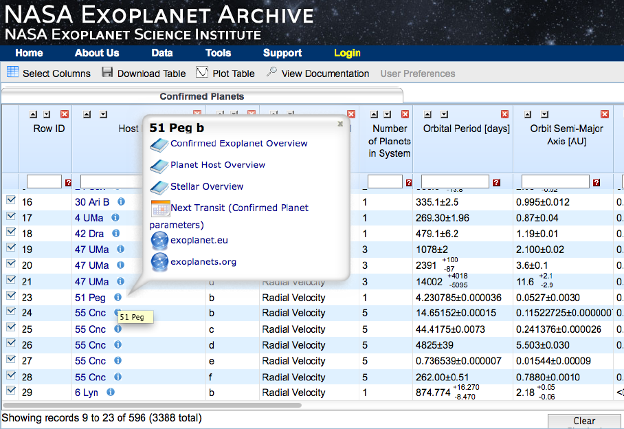
Click on the "Confirmed Exoplanet Overview" item in this pop-up window, and you will see a new page full of LOTS of information about the object.
Included on this page are links to the journal articles which describe the object's discovery, and some subsequent observations as well.
Q 5: What telescope was used to discover 51 Peg b?
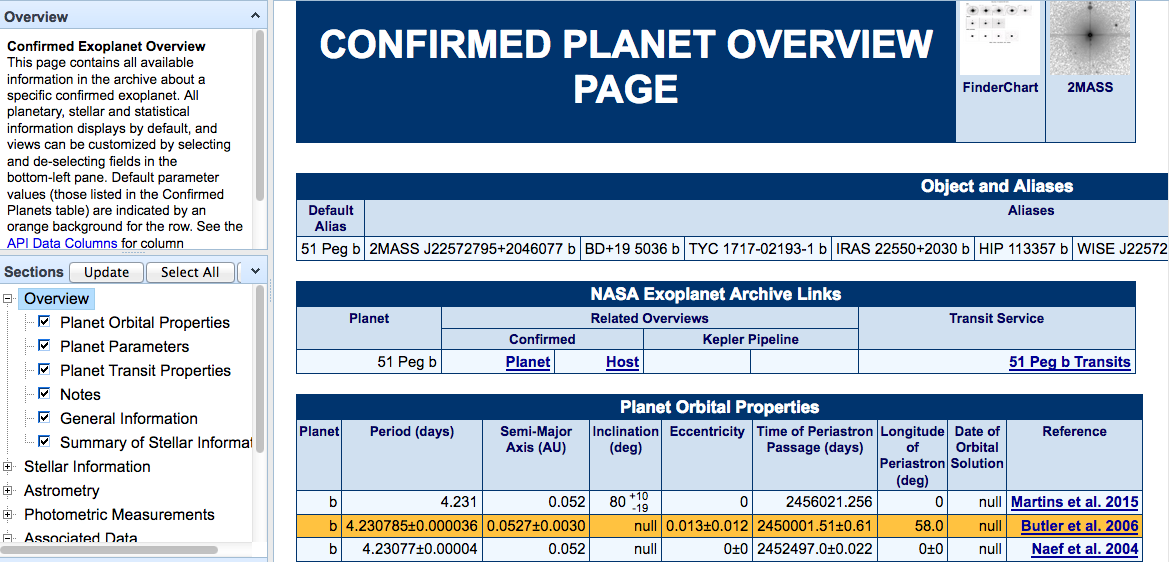
Sometimes, there are even copies of the measurements themselves. Scroll down to the bottom of this page, and look for radial-velocity measurements made by Marcy et al. 1997.
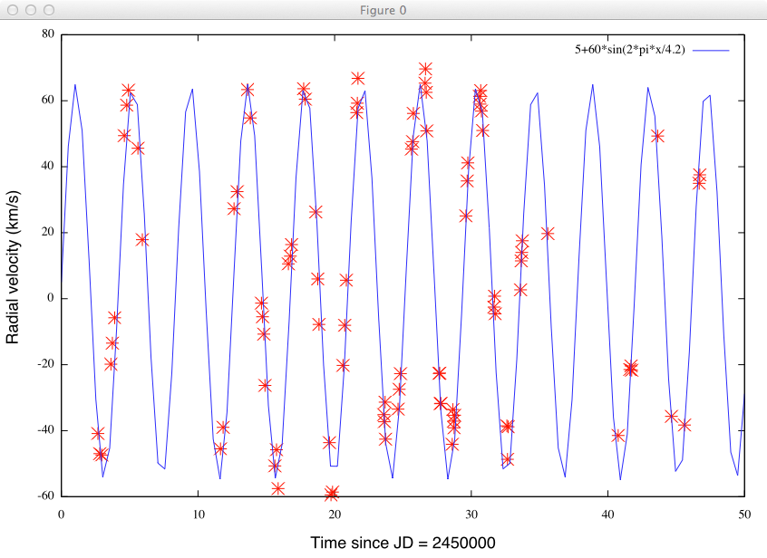
   Q 6:   Make a graph showing the radial velocity of the
          host star, 51 Peg, as a function of time,
          over the period 2450000 to 2450040, using data
          from the Hamilton-Lick collection.


          _Approximately_  how big are the variations in velocity?


          _Approximately_  what is the period of the variations?
If you can't make a graph right now, you can look at my quick-and-dirty graph
Let's try a different discovering technique: imaging, which simply means "taking a picture and seeing a tiny little dot of light next to the host star."
Go back to the the Exoplanet and Candidate Statistics page and click on the item Imaging in the table. It's relatively small, so you should be able to examine all the entries in short time.
   Q 7:   Note that most of the exoplanets in this table have
              either no measured period, or a very large
              uncertainty in the period.

          Why?
Let's pick one of these objects in particular: the exoplanet called 51 Eri b.
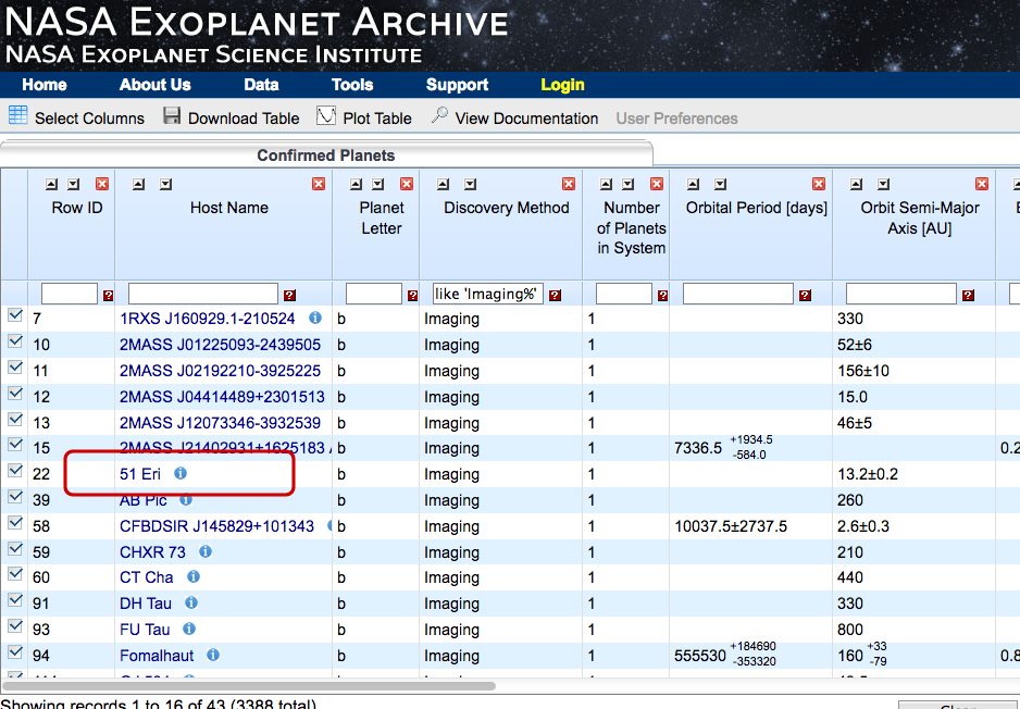
   Q 8:   Based on Macintosh et al. (2015),
          _approximately_ what was the angular separation between
          host star and exoplanet in the discovery images?


   Q 9:   De Rosa et al. (2015) attempt to compute
          an orbit for this exoplanet around 51 Eri.
          The result is not very good because they
          had positions of the object at only ______
          different times.
It was just about one month ago that the European Southern Observatory announced that astronomers using its instruments had found a planet circling the very nearby star Proxima Centauri.
So, what do we know about this planet now?
   Q 10:   Have astronomers measured the following properties
           of Proxima Centauri b?

            a) period

            b) orbital radius

            c) mass

            d) planetary radius
Many people are excited by this particular exoplanet, because it is only about 4.3 light years from Earth. It is not crazy to think that humans could send a probe to this system within the next few hundred years.
Even astronomers have felt this excitement.
   Bonus:   How many papers about Proxima Centauri have been submitted
            to  arXiv  since it was discovered?
Please turn in your answers to these questions before you leave class.
Copyright © Michael Richmond.
This work is licensed under a Creative Commons License.